Problem Formulation
Clarifying the ML Objective
ML framing: Given a real-time context vector of supply, demand, competitor prices, and user signals, the model predicts the price that maximizes a chosen business objective (revenue, GMV, or conversion rate) subject to guardrail constraints.
Before you write a single line of model code, you need to nail down what the business actually wants to optimize. "Maximize revenue" and "maximize conversion rate" sound compatible but they pull in opposite directions. A higher price increases revenue per transaction but kills conversion. A lower price fills every slot but leaves money on the table. The interviewer is testing whether you see this tension immediately.
The ML task type follows directly from your objective. If you're predicting the revenue-maximizing price directly, that's a regression problem. If you're modeling demand elasticity (how does conversion probability change as price increases?), that's also regression but on a different target. If you're choosing among a discrete set of price tiers, it becomes classification or ranking. Get this framing locked in early, because it determines your training labels, your loss function, and your offline evaluation strategy.
"Success" in ML terms is not the same as success in business terms. A model with low RMSE on held-out price predictions might still hurt revenue if it systematically underprices during peak demand. Always connect your offline metric back to the business outcome it proxies for.
Tip: When the interviewer asks "how would you measure success?", give both an offline metric and an online metric. Then explain what gap between them would concern you.
Functional Requirements
Core Requirements
- The model must predict a price (or price multiplier) for a given market zone and request context, with inputs including real-time supply count, demand request rate, time of day, local events, and competitor pricing signals.
- Prices must be updated with sub-minute freshness for ride-hailing and food delivery contexts; stale prices during a demand spike directly cost revenue.
- The system must respect hard price guardrails: a configurable floor and ceiling per market, and a maximum rate-of-change per time window to prevent runaway surge.
- The model must support offline backtesting so new versions can be evaluated on historical data before any live traffic exposure.
- Predictions must be explainable at the feature level; regulators and ops teams need to understand why a price was set, especially in markets with price gouging laws.
Below the line (out of scope)
- User-level personalized pricing (charging different users different prices for the same service). This raises serious fairness and legal concerns and warrants its own scoping conversation.
- Multi-product catalog pricing. Start with a single product category (e.g., standard rides or standard delivery) before generalizing.
- Competitor price prediction. We consume competitor feeds as an input feature; we are not in the business of forecasting what competitors will do next.
Metrics
Offline metrics
Mean Absolute Error (MAE) on price prediction is your primary offline metric. Unlike RMSE, MAE doesn't over-penalize large errors, which matters here because occasional large deviations (e.g., during unusual events) are less catastrophic than systematic small biases. Track it separately per market segment, not just globally.
If you're modeling demand elasticity as a sub-problem, use calibration metrics: does your model's predicted conversion rate at price $X actually match observed conversion rates? A well-calibrated elasticity model is worth more than a low-RMSE price model that gets the shape of the demand curve wrong.
For counterfactual evaluation (covered more in model development), you'll use inverse propensity-weighted metrics to correct for the fact that your training data only contains outcomes at prices the old policy actually served.
Online metrics
- Revenue per session: the primary north star. Captures both price level and conversion jointly.
- Conversion rate: tracks whether higher prices are suppressing demand beyond acceptable levels.
- Take rate (platform fee as a fraction of GMV): useful for marketplace contexts like Uber or Airbnb where the platform earns a percentage.
Guardrail metrics
- Inference latency: p99 must stay under 100ms for real-time serving. If it creeps above that, the pricing service becomes a bottleneck in the request path.
- Price ceiling breach rate: how often does the raw model output exceed the regulatory or business-defined ceiling? A high rate suggests the model is poorly calibrated or the guardrails are too tight.
- Fairness across market segments: prices should not systematically disadvantage users in lower-income zip codes beyond what supply/demand ratios justify. Track average price by demographic proxy and flag anomalies.
Tip: Always distinguish offline evaluation metrics from online business metrics. Interviewers want to see you understand that a model with great AUC can still fail in production.
Constraints & Scale
For a ride-hailing or food delivery context at Uber or DoorDash scale, the numbers look roughly like this:
| Metric | Estimate |
|---|---|
| Prediction QPS | 50,000 to 100,000 (peak, across all markets) |
| Training data size | 500M to 1B labeled request-price-outcome rows per year |
| Model inference latency budget | Under 20ms for model call; 100ms end-to-end including feature fetch |
| Feature freshness requirement | Supply/demand features under 60 seconds; historical features daily |
A few constraints that shape every downstream design decision. First, real-time vs. batch is not a binary choice. You'll likely run a hybrid: pre-computed zone-level prices refreshed every 30 to 60 seconds for the common case, with real-time inference as a fallback for unusual contexts or high-value requests. Second, cold-start is a genuine problem. New market zones have no pricing history, so your model needs a sensible prior (rule-based surge as a fallback) until enough data accumulates. Third, if personalization is ever added to scope, you immediately inherit fairness obligations that require legal review in many jurisdictions.
Common mistake: Candidates jump straight to model architecture without asking whether the pricing decision needs to be explainable. At Uber, Airbnb, and DoorDash, pricing decisions can face regulatory scrutiny. If you can't explain why a price was set, you can't operate in some markets at all.
Data Preparation
Getting your data right is where dynamic pricing systems actually win or lose. A well-tuned model on bad training data will confidently set prices that destroy conversion. Start here.
Data Sources
You're pulling from five distinct source categories, and each has a different freshness profile, reliability story, and failure mode.
Transaction logs are your foundation. Every completed booking, ride, or order gives you a (context, price, outcome) tuple. At Uber scale, this is tens of millions of rows per day. The catch: you only observe outcomes at prices you actually charged. That selection bias will come back to haunt you in the labeling step.
Real-time supply and demand signals include active driver counts, open restaurant capacity, available inventory, and incoming request rates. These are high-frequency, low-latency signals, often arriving as GPS pings or heartbeat events every 5-30 seconds. Volume is enormous (billions of events/day for a large ride-hailing platform), but individual events are cheap and stateless.
Competitor price feeds come from third-party data providers or web scraping pipelines. Freshness is typically 5-30 minutes, and reliability is spotty. Treat these as noisy signals, not ground truth.
Contextual signals include weather APIs, local event calendars (concerts, sports, conferences), and public holiday data. These are low-volume but high-signal for demand spikes. A Taylor Swift concert ending at 11pm in a specific zip code is a meaningful feature.
User session data covers browsing behavior before a purchase: how long someone spent on the pricing screen, whether they compared options, their device type, and their historical acceptance rate at different price points. This is only relevant if personalized pricing is in scope, and you should clarify that with your interviewer early.
Interview tip: When listing data sources, don't just name them. For each one, say what signal it provides, how fresh it needs to be, and what breaks if it goes down. That's what separates a senior answer from a junior one.
Here's a concrete schema for the core transaction event you'd log:
{
  "event_type": "price_accepted",
  "timestamp": "2024-03-15T22:47:03Z",
  "request_id": "req_8f3a2c",
  "market_id": "nyc_manhattan",
  "zone_id": "zone_042",
  "price_offered": 18.50,
  "base_price": 12.00,
  "surge_multiplier": 1.54,
  "model_version": "gbm_v23",
  "features_snapshot": {
    "active_drivers": 142,
    "demand_rate_5m": 89,
    "supply_demand_ratio": 1.60,
    "hour_of_day": 22,
    "is_weekend": true,
    "weather_condition": "rain"
  },
  "outcome": "accepted",
  "revenue": 18.50
}
Log the features snapshot alongside the outcome. Without it, you can't reconstruct what the model saw at decision time, and point-in-time correct training becomes impossible.
Freshness requirements vary dramatically across these sources. Demand signals need sub-minute freshness; a 5-minute-stale supply count during a surge event is useless. Historical elasticity curves, competitor baselines, and user sensitivity scores can be recomputed daily or even weekly without meaningful accuracy loss.
Label Generation
The target variable sounds obvious until you think about it carefully. You want to predict the "optimal price," but you never observe what would have happened at prices you didn't charge.
The most common approach for a supervised baseline is revenue-in-hindsight labeling: for each completed transaction, the label is the actual revenue collected. You train the model to predict expected revenue as a function of price and context, then at inference time, you query the model at several candidate price points and pick the argmax. This sidesteps the counterfactual problem by framing it as a regression task rather than a direct price prediction.
A more sophisticated framing uses demand elasticity labels. For each market zone and time window, you estimate the conversion rate at each price point using historical data, then fit a demand curve. The label becomes the price that maximizes price * P(conversion | price, context). This requires enough price variation in your historical data to estimate the curve, which is a real constraint in new markets.
Warning: Label leakage is one of the most common ML system design mistakes. Always clarify the temporal boundary between features and labels. If your feature snapshot includes any signal computed after the pricing decision (like final trip duration, or post-surge demand recovery), you've leaked the future into training. Your offline metrics will look great and your production model will fail.
Three label quality problems you need to address explicitly:
Selection bias. You only observe outcomes at prices users accepted. Prices that were too high and caused abandonment are missing from your training set. This means your model learns from a biased sample of the demand curve, and will systematically underestimate price sensitivity. Inverse propensity scoring (IPS) is the standard correction: upweight observations from price points that were rarely offered, downweight those that were common.
Delayed feedback. For ride-hailing, the outcome (trip completed, revenue collected) arrives within an hour. For hotel bookings or subscription upgrades, it might take days or weeks. Your labeling pipeline needs to handle this join delay without dropping events or creating gaps in training data.
Promotional noise. Transactions during discount campaigns, referral bonuses, or competitive promotions are outliers. A $5 ride that normally costs $15 doesn't reflect true demand at that price point. Filter these or flag them with a separate feature so the model doesn't learn the wrong elasticity.
The label generation pipeline looks like this:
def generate_training_labels(
    price_decisions: pd.DataFrame,   # (request_id, price_offered, timestamp, features)
    outcomes: pd.DataFrame,          # (request_id, outcome, revenue, outcome_timestamp)
    join_delay_hours: int = 24
) -> pd.DataFrame:
    # Only join outcomes that have had time to materialize
    cutoff = pd.Timestamp.now() - pd.Timedelta(hours=join_delay_hours)
    decisions = price_decisions[price_decisions["timestamp"] < cutoff]

    labeled = decisions.merge(outcomes, on="request_id", how="left")

    # Unmatched = no outcome observed (abandonment or timeout)
    labeled["converted"] = labeled["outcome"] == "accepted"
    labeled["revenue"] = labeled["revenue"].fillna(0.0)

    # Flag promotional transactions for filtering or separate modeling
    labeled["is_promo"] = labeled["surge_multiplier"] < 1.0

    return labeled
Data Processing and Splits
Raw transaction logs are messy. Before anything touches your training pipeline, you need to filter aggressively.
Bot and fraud filtering comes first. Automated requests from scrapers or internal load tests will inflate your demand signal and pollute your training data. Filter by user agent, request rate per session, and known bot IP ranges. For pricing systems specifically, watch for internal QA tools that fire fake pricing requests.
Outlier removal targets transactions at extreme price points, usually from system errors or manual overrides. A $0.01 ride or a $10,000 hotel booking that cleared at 3am are not representative. Use IQR-based filtering per market segment rather than global thresholds, since what's an outlier in a small market might be normal in a dense urban zone.
Deduplication handles retry storms. If a client retries a pricing request three times due to a timeout, you don't want three copies of the same decision in your training set. Deduplicate on request_id before joining with outcomes.
For imbalanced data, the relevant imbalance in pricing is not class imbalance but price point imbalance: most of your data clusters around a narrow band of prices, with sparse coverage at the extremes. Stratified sampling by price bucket during training ensures the model doesn't overfit to the modal price.
Time-based splits are non-negotiable here. Don't use random splits.
If you randomly shuffle and split, your validation set will contain data from the same time periods as your training set. The model will appear to generalize well because market conditions, seasonal patterns, and competitor behavior are shared across splits. In production, you're always predicting the future from the past. Your split should reflect that.
Training:    Jan 1  → Oct 31   (10 months)
Validation:  Nov 1  → Nov 30   (1 month, for hyperparameter tuning)
Test:        Dec 1  → Dec 31   (1 month, held out until final eval)
Use the most recent data for test. If your market has strong seasonality (holiday surge, summer travel peaks), make sure your test window captures a representative period, not just a quiet month.
Data versioning ties everything together. Every training run should be reproducible from a versioned dataset snapshot. Store processed training data as Parquet files on S3 with a date-stamped prefix, and register each snapshot in your feature store's offline catalog. When a model underperforms in production, you need to be able to re-run training on exactly the data that produced it.
s3://pricing-ml/training-data/
  v20240315/
    train.parquet          # Jan–Oct transactions, labeled
    validation.parquet     # Nov transactions
    test.parquet           # Dec transactions
    metadata.json          # feature list, label definition, filter config, row counts
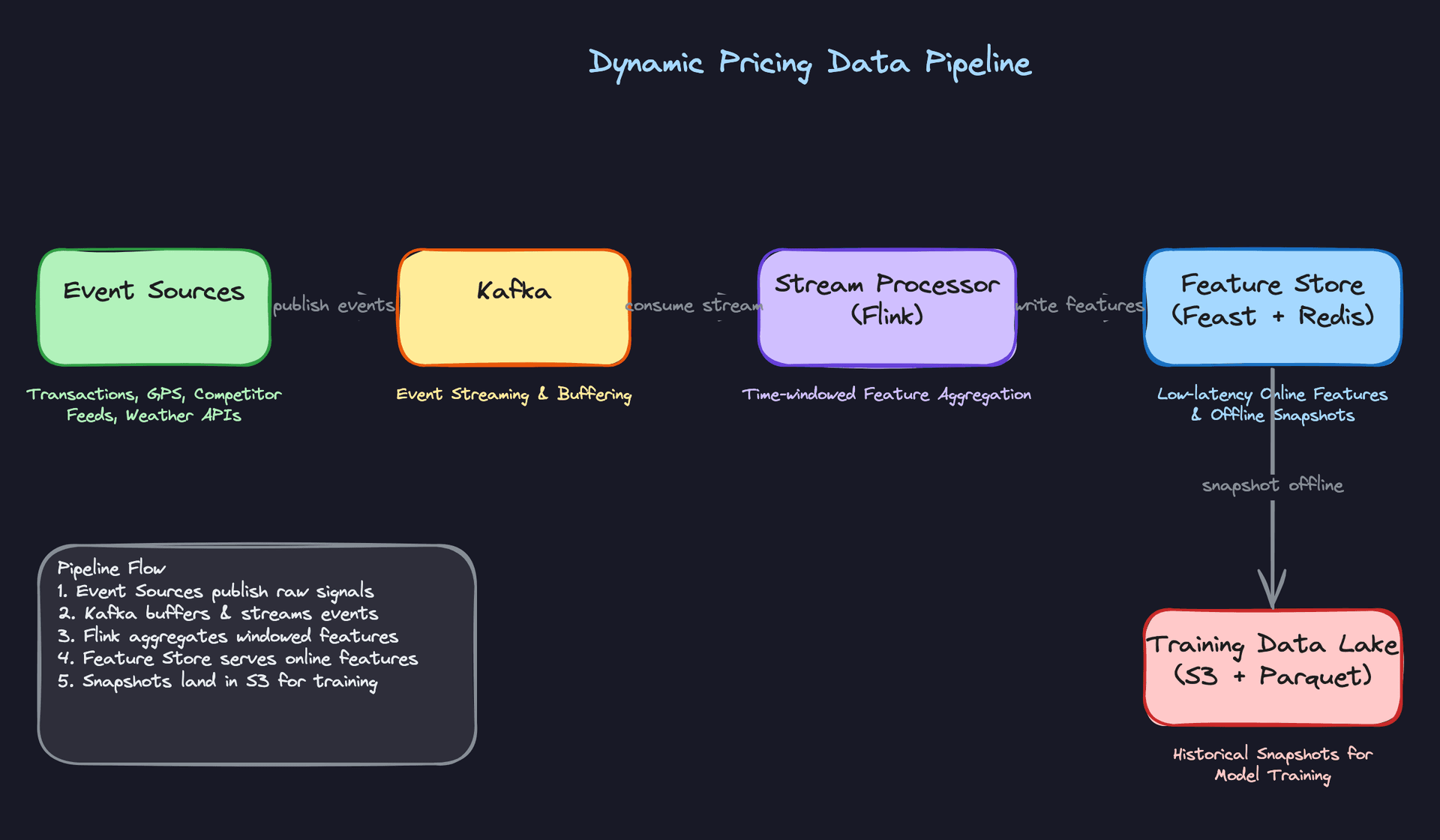
The full pipeline runs two parallel tracks: a streaming path for real-time feature materialization (Kafka to Flink to Redis), and a batch path for training snapshot generation (Spark jobs joining decisions with delayed outcomes, writing versioned Parquet to S3). The feature store (Feast) sits in the middle, providing point-in-time correct retrieval for both online serving and offline training.
Feature Engineering
Good features matter more than model choice here. A gradient boosted tree with sharp supply/demand signals will beat a neural network trained on stale batch features every time. The challenge with dynamic pricing is that you're mixing features with wildly different freshness requirements, from sub-minute streaming aggregates to weekly elasticity curves, and they all need to land in the same feature vector at inference time.
Feature Categories
Supply and Demand Features
These are the heartbeat of any pricing model. Without them, you're just guessing.
| Feature | Type | Computation |
|---|---|---|
active_supply_count | INT | Count of available drivers/listings in zone, updated every 30s via Flink |
demand_request_rate_5m | FLOAT | Rolling count of ride/booking requests in zone over last 5 minutes |
supply_demand_ratio | FLOAT | demand_request_rate / max(active_supply_count, 1), computed at stream time |
demand_rolling_avg_60m | FLOAT | Exponentially weighted average of request rate over 60-minute window |
zone_utilization_pct | FLOAT | Fraction of available supply currently on active trips |
The rolling windows at 5, 15, and 60 minutes each carry different signal. The 5-minute window captures a sudden stadium rush. The 60-minute window gives the model a baseline to compare against. Both matter.
Temporal and Contextual Features
| Feature | Type | Computation |
|---|---|---|
hour_of_day | INT (0-23) | Extracted from request timestamp, localized to market timezone |
is_weekend | BOOL | Derived from request date |
is_local_holiday | BOOL | Joined against a holiday calendar table, updated daily |
nearby_event_attendance | INT | Sum of expected attendance for events within 2km, sourced from event APIs |
weather_severity_score | FLOAT (0-1) | Normalized score from weather API: rain, snow, and wind combined |
Don't underestimate the event attendance feature. A 50,000-person concert ending at 11pm is one of the strongest demand signals you have, and it's knowable hours in advance.
Market and Competitive Features
| Feature | Type | Computation |
|---|---|---|
competitor_price_index | FLOAT | Ratio of your price to median competitor price in zone, refreshed every 5 minutes |
historical_price_elasticity | FLOAT | Estimated % demand change per % price change, computed weekly per market segment |
surge_multiplier_history_24h | FLOAT | Average surge multiplier applied in this zone over the last 24 hours |
market_segment_baseline_price | FLOAT | Rolling 7-day median accepted price for this zone/product type |
Elasticity is a batch feature. It doesn't change minute to minute, and computing it requires enough historical transactions to be statistically meaningful. Weekly recomputation per zone is usually sufficient.
User and Trip Features (When Personalization Is in Scope)
Note: User-level pricing is legally restricted in some jurisdictions. Confirm with your interviewer whether personalization is in scope before designing these features.
| Feature | Type | Computation |
|---|---|---|
user_price_sensitivity_score | FLOAT (0-1) | Logistic regression output trained on historical acceptance/rejection at different price points |
estimated_trip_distance_km | FLOAT | Computed at request time from origin/destination using routing service |
user_acceptance_rate_at_surge | FLOAT | Fraction of past requests accepted when price was above 1.2x baseline, 90-day window |
user_lifetime_trips | INT | Total completed trips, updated daily in batch |
The acceptance rate at surge is particularly useful. A user who has accepted 2x prices 80% of the time in the past is a different signal than one who cancels the moment surge kicks in.
Feature Computation
Batch Features
Elasticity scores, user sensitivity scores, market baselines, and lifetime trip counts all live here. These run as daily Spark jobs against your data warehouse, writing outputs into the offline feature store.
# PySpark: compute 90-day user acceptance rate at surge
from pyspark.sql import functions as F

user_surge_acceptance = (
    transactions
    .filter(F.col("price_multiplier") > 1.2)
    .groupBy("user_id")
    .agg(
        F.count("*").alias("surge_requests"),
        F.sum(F.when(F.col("status") == "completed", 1).otherwise(0))
         .alias("surge_acceptances")
    )
    .withColumn(
        "acceptance_rate_at_surge",
        F.col("surge_acceptances") / F.col("surge_requests")
    )
)

# Write to offline store and materialize to Redis via Feast
user_surge_acceptance.write.parquet("s3://features/user_surge_acceptance/")
The Spark job writes Parquet to S3. Feast picks it up, registers it against the feature schema, and materializes it to Redis for online serving. That materialization step is where skew gets introduced if you're not careful (more on that below).
Near-Real-Time Features
Supply count, demand rate, and rolling windows need to reflect what's happening right now. A 10-minute-old supply count is useless when a surge is starting.
# Flink: compute 5-minute rolling demand rate per zone
from pyflink.datastream import StreamExecutionEnvironment
from pyflink.table import StreamTableEnvironment

env = StreamExecutionEnvironment.get_execution_environment()
t_env = StreamTableEnvironment.create(env)

t_env.execute_sql("""
    CREATE TABLE demand_events (
        zone_id     STRING,
        event_time  TIMESTAMP(3),
        WATERMARK FOR event_time AS event_time - INTERVAL '10' SECOND
    ) WITH (
        'connector' = 'kafka',
        'topic' = 'ride_requests',
        'format' = 'json'
    )
""")

t_env.execute_sql("""
    INSERT INTO feature_store_sink
    SELECT
        zone_id,
        COUNT(*) AS demand_request_rate_5m,
        TUMBLE_END(event_time, INTERVAL '5' MINUTE) AS window_end
    FROM demand_events
    GROUP BY zone_id, TUMBLE(event_time, INTERVAL '5' MINUTE)
""")
Flink writes these aggregates directly to Redis with a TTL of 10 minutes. If the key expires before the next window fires, the pricing service falls back to the last known value rather than failing.
Real-Time Features
A small number of features can only be computed at request time. Trip distance is the clearest example: you don't know the origin/destination pair until the user opens the app.
# Called synchronously during the pricing request
def compute_realtime_features(request: PricingRequest) -> dict:
    distance_km = routing_service.estimate_distance(
        origin=request.pickup_lat_lng,
        destination=request.dropoff_lat_lng
    )
    duration_min = routing_service.estimate_duration(
        origin=request.pickup_lat_lng,
        destination=request.dropoff_lat_lng,
        departure_time=request.timestamp
    )
    return {
        "estimated_trip_distance_km": distance_km,
        "estimated_trip_duration_min": duration_min,
    }
Keep this list short. Every synchronous call at serving time adds latency. If a feature can be precomputed, precompute it.
Feature Store Architecture
The feature store has two jobs that seem simple but conflict with each other: serve features fast at inference time, and serve the exact same features during training. Most teams get the first part right and quietly fail at the second.
┌─────────────────────────────────────────────────────────────────────────┐
│                        FEATURE PIPELINE                                 │
│                                                                         │
│  ┌──────────────┐    ┌─────────────────┐    ┌─────────────────────┐    │
│  │  Ride Events │    │  Batch Sources  │    │  External APIs      │    │
│  │  (Kafka)     │    │  (Data Warehouse│    │  (Weather, Events,  │    │
│  │              │    │   / S3)         │    │   Competitor Prices)│    │
│  └──────┬───────┘    └────────┬────────┘    └──────────┬──────────┘    │
│         │                    │                         │               │
│         ▼                    ▼                         ▼               │
│  ┌──────────────┐    ┌─────────────────┐    ┌─────────────────────┐    │
│  │  Flink       │    │  Spark          │    │  Ingestion Jobs     │    │
│  │  Streaming   │    │  Batch Jobs     │    │  (hourly/daily)     │    │
│  │  (5m windows)│    │  (daily)        │    │                     │    │
│  └──────┬───────┘    └────────┬────────┘    └──────────┬──────────┘    │
│         │                    │                         │               │
│         │            ┌───────▼─────────────────────────▼──────┐        │
│         │            │         OFFLINE STORE                  │        │
│         │            │    S3 + Hive / Parquet                 │        │
│         │            │    (partitioned by date, point-in-time │        │
│         │            │     correct joins for training)        │        │
│         │            └───────────────────┬────────────────────┘        │
│         │                                │                             │
│         │                    ┌───────────▼────────────┐               │
│         └───────────────────►│      ONLINE STORE      │               │
│          (direct write,      │      Redis             │               │
│           TTL = 10 min)      │      (p99 < 5ms reads) │               │
│                              └───────────┬────────────┘               │
│                                          │  Feast materializes         │
│                                          │  batch features on schedule │
│                                          ▼                             │
│                              ┌───────────────────────┐                │
│                              │    PRICING SERVICE    │                │
│                              │  (online inference)   │                │
│                              └───────────────────────┘                │
└─────────────────────────────────────────────────────────────────────────┘
Two paths feed the online store. Flink writes streaming aggregates directly to Redis with a short TTL, bypassing the offline store entirely for latency reasons. Batch features take the longer route: Spark writes Parquet to S3, Feast registers the schema and materializes to Redis on a schedule. Both paths converge at the same Redis keyspace, so the pricing service sees a single unified feature vector regardless of where each value came from.
The offline store is not just an archive. It's the source of truth for training. Every feature write lands here, partitioned by date, so that point-in-time correct joins are possible when you generate training examples later.
Online store (Redis): Batch features are materialized here by Feast on a schedule. Streaming features are written directly by Flink. Every key has a TTL. The pricing service reads from Redis with a p99 target under 5ms. If a key is missing (new market, cold start), the service falls back to market-level defaults rather than blocking.
Offline store (S3 + Hive/Parquet): Every feature write also lands here, partitioned by date. This is what training jobs read from. The critical requirement is point-in-time correctness: when you're building a training example for a transaction that happened at 2:15pm on March 3rd, you need the feature values as they existed at 2:15pm on March 3rd, not the values from the end-of-day snapshot.
# Feast point-in-time correct join for training data generation
from feast import FeatureStore

store = FeatureStore(repo_path=".")

# entity_df has columns: user_id, zone_id, event_timestamp
training_df = store.get_historical_features(
    entity_df=transaction_events,
    features=[
        "user_features:user_price_sensitivity_score",
        "user_features:acceptance_rate_at_surge",
        "zone_features:supply_demand_ratio",
        "zone_features:demand_request_rate_5m",
        "zone_features:competitor_price_index",
    ]
).to_df()
Without the point-in-time join, you're accidentally training on future feature values. The model looks great offline and falls apart in production. This is one of the most common ways pricing models fail silently.
Key insight: The most common failure mode in ML systems is training-serving skew. Features computed differently in batch training vs. online serving will cause your model to behave in production exactly as it did in training, just on a different distribution than you think. Always design for consistency: one feature definition, two materialization paths.
One practical guard: log the actual feature vector used at inference time alongside the pricing decision. Then, periodically sample those logged vectors and compare them against what your offline pipeline would have produced for the same timestamp. Any divergence is skew. Catching it early, before it contaminates your training data, saves enormous debugging time later.
Model Selection & Training
The model you choose for pricing isn't just a technical decision. It's a statement about how much uncertainty you're willing to accept, how fast your market moves, and whether you trust your historical data to reflect the prices you haven't tried yet.
Model Architecture
Start with the simplest thing that could work, then build up. In an interview, walking through all three tiers shows the interviewer you understand the tradeoffs, not just the state of the art.
Approach 1: Rule-Based Surge Multiplier
This is your baseline. It's not glamorous, but Uber ran something close to this in production for years.
The logic is a lookup table: compute the supply-demand ratio for a geographic zone, bucket it, and return a fixed multiplier. Demand 2x supply? Price goes to 1.5x. Demand 3x supply? Price goes to 2.0x.

The input is a single ratio. The output is a discrete multiplier from a predefined set. No training required, fully explainable, and trivial to audit. When a regulator asks why a price spiked during a hurricane, you can point to a spreadsheet.
The failure mode is obvious: the multiplier thresholds are hand-tuned and don't generalize. A zone near a stadium behaves differently from an airport zone, and a fixed table can't capture that. You also can't optimize for revenue or conversion rate directly; you're just reacting to a ratio.
Tip: Always propose this as your baseline in the interview, even if you plan to go further. It shows you value explainability and have a fallback if the ML system fails.
Approach 2: Gradient Boosted Regression
This is the production workhorse for most pricing systems. XGBoost or LightGBM trained on historical transactions, predicting the revenue-maximizing price given a feature vector.

Input features and dimensions:
feature_vector = {
    # Supply/demand (real-time, from Redis)
    "supply_count_zone":         float,   # active drivers/listings in zone
    "demand_rate_5min":          float,   # requests per minute, 5-min window
    "supply_demand_ratio":       float,   # derived ratio
    "supply_demand_ratio_15min": float,   # smoothed version

    # Temporal (deterministic)
    "hour_of_day":               int,     # 0-23
    "day_of_week":               int,     # 0-6
    "is_holiday":                bool,
    "minutes_to_event_nearby":   float,   # nearest concert/game, null if none

    # Market context (batch-computed daily)
    "competitor_price_index":    float,   # normalized competitor price
    "historical_elasticity":     float,   # price sensitivity for this zone/segment
    "baseline_price":            float,   # zone's 30-day median price

    # Weather (external API)
    "precipitation_mm":          float,
    "temperature_celsius":       float,
}
Architecture choice: Tree-based models are the right call here for several reasons. Pricing data is tabular, features have non-linear interactions (demand at 2am behaves differently than demand at 8pm even at the same ratio), and you need fast inference without GPU infrastructure. LightGBM can serve a prediction in under 5ms on CPU.
Loss function: You have two options depending on how you frame the target.
If you're predicting price directly, use MAE or Huber loss. MAE is more robust to outlier transactions from promotions or anomalous events. Huber gives you a smooth gradient near zero while being outlier-resistant at the tails.
If you're predicting conversion probability at a given price (the elasticity framing), use log loss. Then you find the price that maximizes price * P(conversion | price, context) analytically or via a small grid search.
The elasticity framing is more principled. It separates "what price will people accept" from "what price should we charge," which makes the system easier to reason about and debug.
Output: A single float representing the recommended price, in dollars. Before this leaves the model, it passes through an elasticity calibrator that adjusts the raw prediction using the estimated demand curve, then through guardrails that enforce floor/ceiling constraints.
Approach 3: Contextual Bandit for Closed-Loop Optimization
The fundamental problem with supervised models is that they're trained on prices that were actually charged. You've never observed what would have happened if you'd charged 20% more in that zone at that time. Your training data has a massive selection bias baked in.
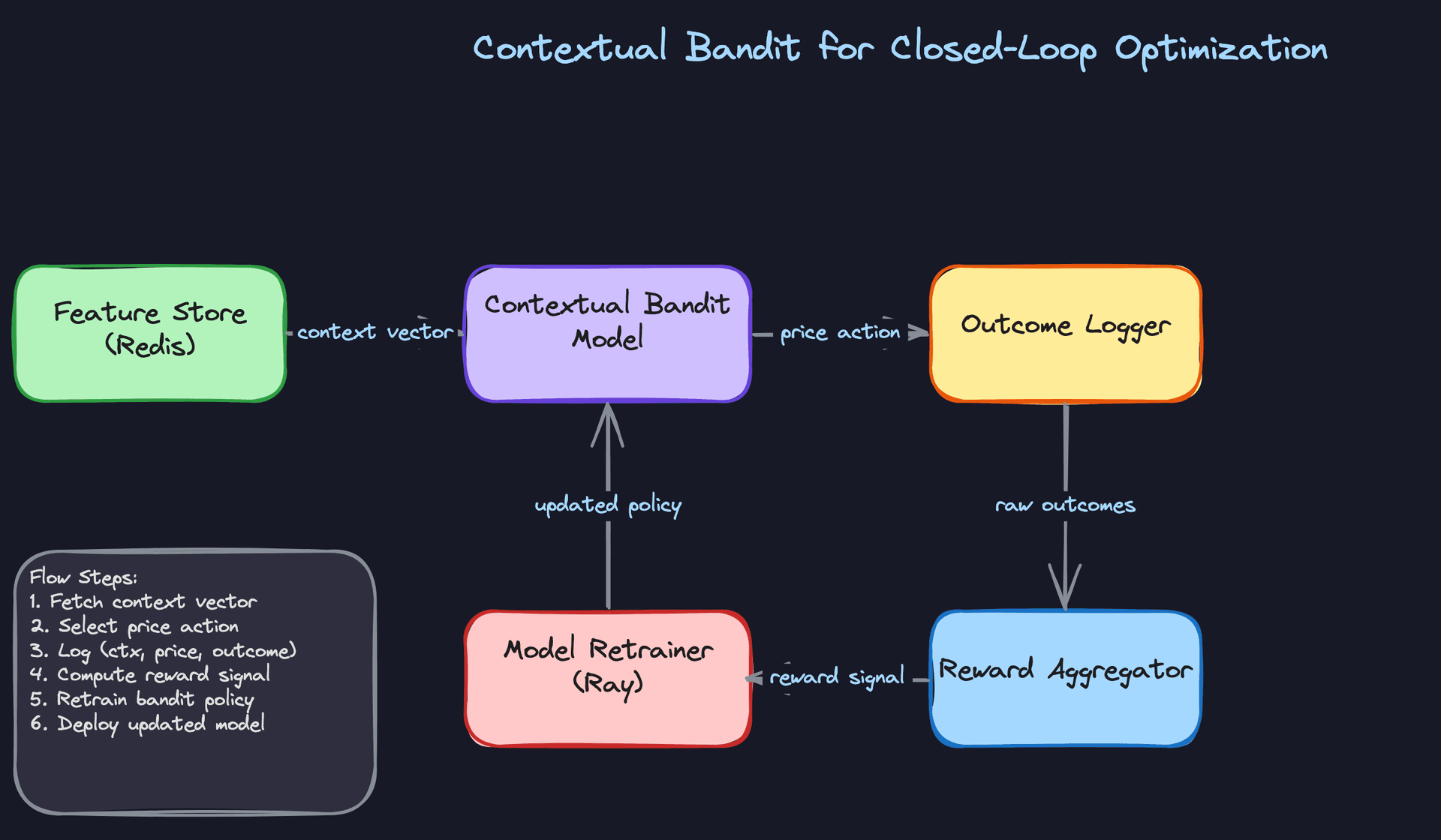
A contextual bandit treats each pricing decision as an action and learns from the reward (conversion, revenue) that follows. At inference time, it balances exploiting the best-known price for a context against exploring nearby price points to reduce uncertainty.
Input: The same feature vector as the GBM, plus an uncertainty estimate for the current context. The bandit needs to know how much it already knows about this situation.
Architecture choice: LinUCB (linear upper confidence bound) is a reasonable starting point. It's interpretable, has theoretical guarantees, and trains incrementally. For more complex contexts, a neural contextual bandit (a small neural network with a UCB or Thompson sampling head) can capture non-linear interactions while still exploring.
Reward signal: This is where it gets tricky. The reward (did the user convert? what was the revenue?) arrives with a delay, sometimes minutes for ride-hailing, hours for e-commerce. Your reward aggregator needs to join price decisions to outcomes and handle late arrivals gracefully.
The guardrails problem. Without constraints, a bandit will explore prices that are technically valid but terrible for the business: charging $200 for a $15 ride to see what happens. You need hard price bounds, rate-of-change limits, and a minimum exploration budget that doesn't let the bandit concentrate all exploration in low-traffic periods.
Key insight: The exploration-exploitation tradeoff isn't just a modeling concern. It's a product and legal concern. Any price you charge to a real user is a real price. Your exploration strategy needs sign-off from product and legal, not just the ML team.
Training Pipeline
Infrastructure
The GBM baseline trains on CPU and finishes in under an hour even on 6 months of transaction data. You don't need a GPU cluster for this. A single large memory instance (128GB RAM) running LightGBM with 32 threads is enough for most markets.
The contextual bandit is different. If you're using a neural bandit, you'll want GPU training, and you'll want it to run frequently, potentially every few hours, to incorporate recent reward signals. Ray Tune handles distributed hyperparameter search well here, and Ray Train handles the distributed training itself.
# LightGBM training config for pricing regression
import lightgbm as lgb

params = {
    "objective":         "regression_l1",  # MAE loss, robust to outliers
    "num_leaves":        127,
    "learning_rate":     0.05,
    "feature_fraction":  0.8,
    "bagging_fraction":  0.8,
    "bagging_freq":      5,
    "min_child_samples": 50,               # prevents overfitting on sparse zones
    "n_estimators":      1000,
}

model = lgb.train(
    params,
    train_data,
    valid_sets=[val_data],
    callbacks=[lgb.early_stopping(50), lgb.log_evaluation(100)],
)
Training Schedule and Data Windowing
For fast-moving markets like ride-hailing or food delivery, retrain daily on a rolling 90-day window. Beyond 90 days, older data starts to hurt more than it helps; pricing patterns from last summer don't reflect today's competitive landscape.
For stable markets (e-commerce catalog pricing), weekly retraining on a 6-month window is usually sufficient.
The windowing decision matters more than most candidates realize. Too short a window and you lose rare but important patterns (holiday surges, major events). Too long and you're training on a market that no longer exists.
Incremental retraining (fine-tuning on recent data) is faster but risks catastrophic forgetting of rare events. Full retraining is safer and, for tree models, cheap enough that there's no reason not to do it.
Hyperparameter Tuning
Run a full Optuna or Ray Tune sweep when you first deploy a new model architecture. After that, use a narrow search around the known-good configuration on each retrain cycle. A full sweep on every daily retrain is wasteful and can introduce instability if a new configuration overfits to a recent anomaly.
import optuna

def objective(trial):
    params = {
        "num_leaves":        trial.suggest_int("num_leaves", 31, 255),
        "learning_rate":     trial.suggest_float("learning_rate", 0.01, 0.1, log=True),
        "feature_fraction":  trial.suggest_float("feature_fraction", 0.6, 1.0),
        "min_child_samples": trial.suggest_int("min_child_samples", 20, 100),
    }
    model = train_lgbm(params, train_data)
    return evaluate_mae(model, val_data)

study = optuna.create_study(direction="minimize")
study.optimize(objective, n_trials=100)
Offline Evaluation
"It has good MAE" is not enough. Your interviewer will push back, and they should.
Metrics
Start with MAE on held-out price predictions, but immediately connect it to business impact. A $0.50 MAE in a $15 ride market is meaningful. The same MAE in a $200 hotel market is noise.
The metrics that actually matter:
- Revenue per session: Does the model's recommended price, when applied, generate more revenue than the baseline?
- Conversion rate at recommended price: Are users accepting the price at the expected rate?
- Elasticity accuracy: Does the model's predicted demand curve match observed conversion rates across price points? This is the hardest metric to compute and the most important.
Evaluation Methodology
Use time-based splits, not random splits. If you randomly shuffle your training and test data, you'll leak future information into training and get optimistic metrics that don't hold in production. Your test set should always be the most recent time period.
# Time-based train/val/test split
train = transactions[transactions.date < "2024-09-01"]
val   = transactions[(transactions.date >= "2024-09-01") &
                     (transactions.date < "2024-10-01")]
test  = transactions[transactions.date >= "2024-10-01"]
For backtesting, replay historical pricing decisions through your new model and compare the predicted prices to what was actually charged, then estimate the revenue delta using the observed elasticity curve. This is imperfect because you can't observe counterfactual outcomes, but it's the best you can do offline.
Counterfactual Evaluation and Selection Bias
This is where most candidates lose points. Your training data only contains transactions that happened at the prices you actually charged. You never observe what would have happened at a different price. This is selection bias, and it makes your demand elasticity estimates unreliable.
Inverse propensity scoring (IPS) is the standard correction. For each observed transaction, you weight it by the inverse probability that the pricing policy would have chosen that price. Transactions at prices the policy rarely chose get upweighted; transactions at the policy's favorite prices get downweighted.
# Simplified IPS weighting for elasticity estimation
def compute_ips_weights(observed_prices, policy_probabilities):
    """
    observed_prices:      array of prices that were actually charged
    policy_probabilities: P(price | context) under the logging policy
    """
    # Clip to avoid extreme weights from near-zero probabilities
    clipped_probs = np.clip(policy_probabilities, a_min=0.01, a_max=None)
    weights = 1.0 / clipped_probs
    # Normalize to prevent high-variance estimates
    return weights / weights.mean()
In practice, IPS has high variance when the logging policy is very concentrated (it almost always charged the same price). Doubly robust estimators (combining IPS with a direct model) reduce variance at the cost of some bias.
Error Analysis
Your model will make systematic mistakes in specific slices. Find them before your interviewer does.
New markets with sparse data will have the highest error. The model has seen very few transactions from a market that launched last month, so its elasticity estimates are essentially guesses. Flag these markets and fall back to the rule-based baseline until you have enough data.
Rare events (concerts, sports finals, natural disasters) are underrepresented in training data almost by definition. Your model will underestimate demand during these events. The fix is to inject event-aware features and, for known upcoming events, to use the rule-based multiplier as an override.
Competitive price changes are a lagging signal. If a competitor drops prices by 30% overnight, your model won't know until the next batch feature computation. Monitor for sudden conversion rate drops as an early warning signal.
Common mistake: Candidates evaluate pricing models purely on prediction accuracy and skip the business metric connection. An interviewer at Uber or Airbnb will immediately ask "so what does a 0.3 improvement in MAE mean for revenue?" If you can't answer that, the evaluation section falls apart.
Online Evaluation
Offline metrics tell you the model is plausible. Online experiments tell you it actually works.
Standard A/B tests have a contamination problem for pricing. If you charge treatment users higher prices, some of them will switch to control zones or time periods, inflating the control group's apparent performance. The treatment effect leaks.
Switchback experiments solve this by splitting on time rather than users. For 10 minutes, the entire market runs on the new model. For the next 10 minutes, it reverts to the baseline. You compare revenue per minute across treatment and control windows.
The tradeoff is that switchback experiments require longer run times to achieve statistical significance, since each time window is one observation rather than each user being one observation. For high-traffic markets, this is fine. For low-traffic markets, you may need to run for weeks.
Tip: When the interviewer asks how you'd validate the model in production, don't just say "A/B test." Explain why geographic or user-level splits create interference in a marketplace, and propose switchback experiments. That's the answer that lands at Uber, Airbnb, and DoorDash.
Inference & Serving
Pricing is one of the few ML systems where latency directly affects revenue. A slow price response on a ride-hailing app means the user sees a spinner, gets frustrated, and cancels. A stale price on a food delivery app means you're either leaving money on the table or losing the order entirely. Getting serving right here isn't an afterthought.
Serving Architecture
Online vs. pre-computed: the real decision
The first question isn't which model to use. It's whether you need per-request inference at all.
For ride-hailing and food delivery, prices are highly contextual: they depend on the exact pickup zone, the current driver count, and what's happening right now. Pre-computing every combination is impractical, so you need real-time inference with a sub-100ms budget. For e-commerce catalog pricing, you have a finite set of SKUs and market segments. You can run a batch job every 15 minutes, push prices into Redis, and serve them as cache lookups. The model never sits in the critical path.
In practice, most production systems use both. Real-time inference handles the long tail of novel contexts; the pre-computed cache handles the high-volume, predictable cases.
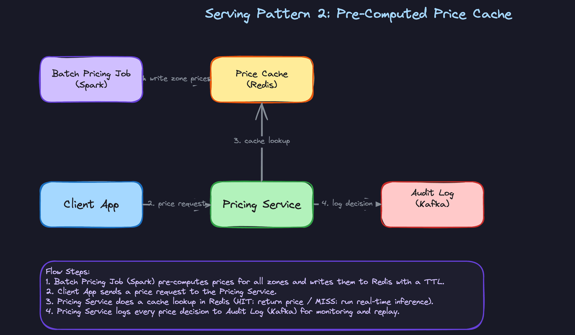
Key insight: Pre-computed prices can serve 95% of requests with zero model latency. Real-time inference handles the edge cases. Design for both from day one.
Model serving infrastructure
For a gradient boosted model (XGBoost/LightGBM), you don't need a GPU server. These models run fast on CPU, and a single core can handle thousands of inferences per second. Wrap the model in a lightweight FastAPI service, containerize it, and deploy behind a load balancer. Simple, cheap, and easy to reason about.
If you move to a neural network for demand forecasting or a contextual bandit, Triton Inference Server becomes worth the operational overhead. Triton handles model versioning, batching, and multi-framework support (TensorFlow, PyTorch, ONNX) in one place. It also exposes gRPC endpoints, which shave latency compared to REST when you're calling from an internal service.
Don't reach for GPU serving unless your model actually needs it. A tree-based model on a GPU is slower than on CPU because the workload doesn't parallelize the way matrix ops do.
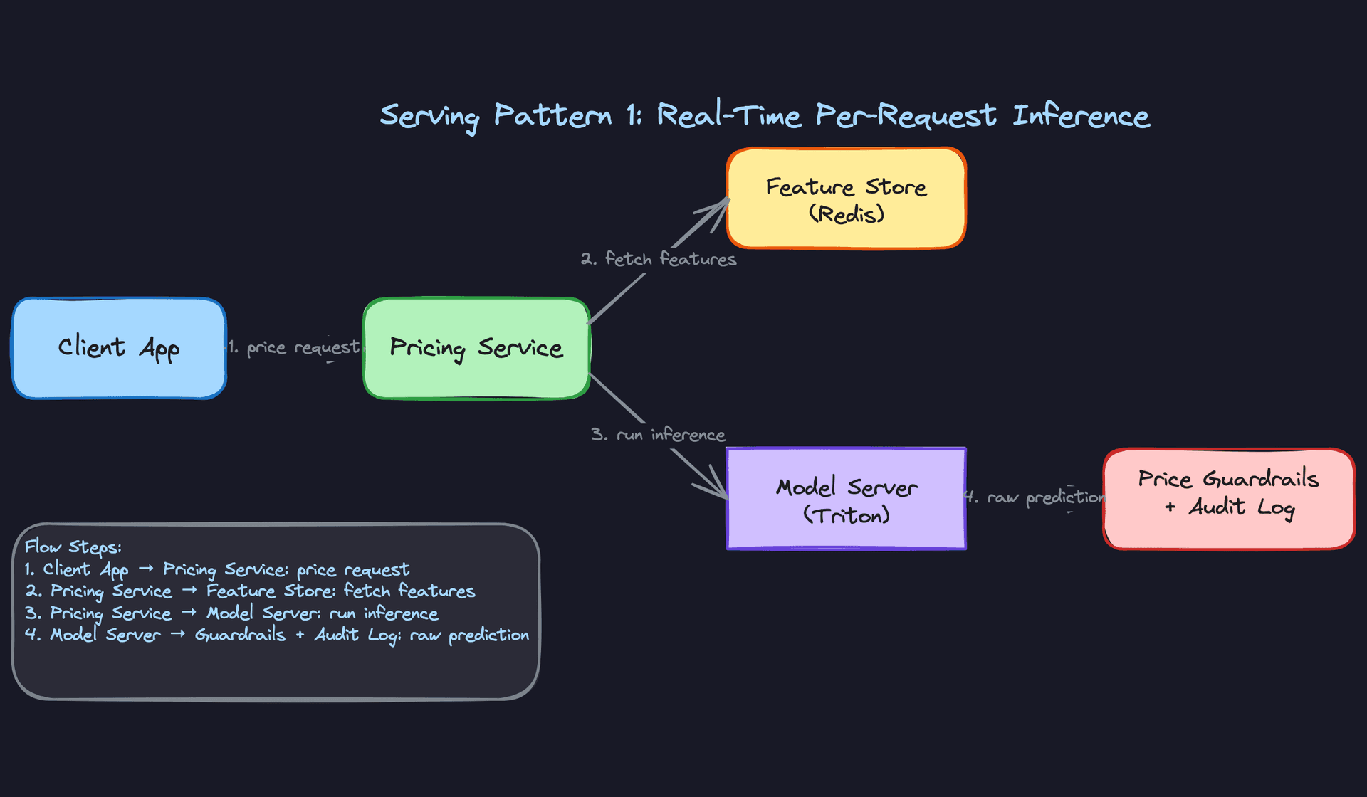
End-to-end request flow
When a pricing request comes in, here's what actually happens:
- The Pricing Service receives the request with context (zone ID, user ID, timestamp).
- It fires a parallel fetch to Redis for the feature vector (supply count, demand rate, rolling windows, competitor index).
- The assembled feature vector goes to the model server via gRPC.
- The model returns a raw price prediction.
- The Pricing Service runs post-processing: apply elasticity calibration, enforce floor/ceiling guardrails, round to a presentable price point.
- The final price is returned to the caller and the decision is logged to Kafka for monitoring.
Steps 2 and 3 can run concurrently if you have features from multiple stores. That's worth doing; it's free latency savings.
Latency breakdown
Target budget for a real-time pricing call: 100ms end-to-end.
| Stage | Typical latency | Notes |
|---|---|---|
| Feature fetch (Redis) | 1-3ms | Single round-trip, co-located |
| Model inference (CPU, GBM) | 5-15ms | Depends on tree depth and feature count |
| Model inference (Triton, NN) | 10-30ms | With batching; higher for single requests |
| Post-processing + guardrails | 1-2ms | In-process, negligible |
| Network + serialization | 5-20ms | gRPC is faster than REST here |
If you're blowing the budget, the culprit is almost always feature fetch latency from a cold cache or a slow downstream call. Profile before optimizing the model.
Optimization
Model optimization
For tree-based models, the main lever is reducing tree depth and feature count. Profile which features contribute least to accuracy and drop them. Fewer features means faster inference and a smaller Redis payload.
For neural models, quantization is your first move. Converting from FP32 to INT8 typically cuts inference time by 2-4x with minimal accuracy loss on pricing tasks. You can do this post-training with ONNX Runtime or Triton's built-in quantization support. Distillation (training a smaller model to mimic a larger one) is worth considering if you're running a complex ensemble and need to hit aggressive latency targets.
Common mistake: Candidates jump to quantization and distillation before profiling. In most pricing systems, the bottleneck is feature fetch, not model inference. Measure first.
Batching
Batching matters when you're serving many concurrent requests. Triton supports dynamic batching: it holds requests for a configurable window (say, 5ms) and groups them into a single inference call. This dramatically improves GPU utilization and throughput at the cost of a small latency increase per request.
For CPU-based GBM serving, batching is less impactful because tree inference doesn't benefit from vectorization the same way. Focus on horizontal scaling instead.
GPU vs. CPU
Tree models: CPU, always. Neural models with large embedding tables or transformer architectures: GPU. The break-even point is roughly when your model has more than a few million parameters and you're serving at high QPS. Below that, the overhead of GPU memory transfers and driver latency makes CPU faster for individual requests.
Fallback strategies
Your model will go down. Plan for it.
The cleanest fallback is the pre-computed price cache. If the model server is unavailable or exceeds a latency threshold (say, 80ms), the Pricing Service falls back to the last cached price for that zone. This is almost always acceptable; a 15-minute-old price is better than a 500ms timeout.
If the cache is also stale, fall back to the rule-based surge multiplier. It's deterministic, fast, and requires no external calls. Every ML pricing system should keep the rule-based system alive as an emergency fallback, not just for launch but permanently.
Set a circuit breaker on the model server call. If it fails 5 times in 10 seconds, open the circuit and route to fallback automatically. Don't wait for an on-call engineer to notice.
Online Evaluation & A/B Testing
Running A/B tests on pricing models
Pricing A/B tests are harder than typical product experiments because prices affect both sides of the marketplace. If you raise prices in the treatment group, some users switch to the control group's lower price. This spillover contaminates your results.
The standard fix for ride-hailing and delivery is geo-based splitting: assign entire cities or zones to treatment or control, not individual users. This eliminates cross-group contamination but reduces statistical power because you have fewer independent units.
For markets where geo-splitting isn't practical, switchback experiments work well. Alternate treatment and control on a time-based schedule (e.g., treatment for 30 minutes, control for 30 minutes) within the same zone. You lose some sensitivity to time-of-day effects, but you avoid spillover entirely.
Interview tip: If you just say "random user split," the interviewer will push back on marketplace interference. Mention geo-splits or switchback experiments proactively. It signals you've thought about this in production, not just in theory.
Online metrics and statistical methodology
Primary metrics: revenue per session, conversion rate (request to booking), and take rate. Secondary metrics: driver/host earnings (to catch cases where you're winning revenue by squeezing supply), and cancellation rate (a leading indicator that prices are too high).
Use a sequential testing framework (like mSPRT) rather than waiting for a fixed sample size. Pricing experiments move fast and you want to be able to call them early without inflating false positive rates. Set your minimum detectable effect before the experiment starts; a 1% revenue lift at Uber's scale is worth detecting, but you need to size the experiment accordingly.
Watch for novelty effects in the first 24-48 hours. Users sometimes behave differently when prices change simply because the change is new. Don't call the experiment in the first day.
Ramp-up and rollback
Start at 1% of traffic. Monitor for 24 hours. If conversion rate and revenue per session are within acceptable bounds, ramp to 5%, then 10%, then 50%, then 100%. Each step should have a hold period and automated checks.
Define rollback triggers before you start the experiment, not after you see bad numbers. Typical triggers: conversion rate drops more than 5% relative to control, p99 latency exceeds 200ms, or the circuit breaker fires more than 10 times per minute. Automate the rollback; don't rely on someone being awake to pull the lever.
Interleaving
Interleaving is primarily useful for ranking systems (search, recommendations) where you can show results from two models to the same user in the same session and measure which items get clicked. For pricing, you can't show two prices simultaneously, so interleaving doesn't apply directly. Skip this in your interview answer unless the interviewer specifically asks about catalog ranking within a pricing context.
Deployment Pipeline
Key insight: The deployment pipeline is where most ML projects fail in practice. A model that can't be safely deployed and rolled back is a model that won't ship.
Validation gates
Before a new model version touches production traffic, it has to pass a gauntlet of automated checks. The minimum bar:
- Offline accuracy regression: the new model's MAE on a held-out validation set must not exceed the current production model's MAE by more than a defined threshold (say, 2%).
- Price distribution check: compare the distribution of predicted prices from the new model against the current model on the same input set. A sudden shift in the mean or tail is a red flag even if aggregate MAE looks fine.
- Latency benchmark: run the model under simulated load and confirm p99 latency stays within budget.
- Schema validation: confirm the model accepts the current feature schema. A feature rename or type change that slips through here will cause silent failures in production.
None of these gates should require a human to approve. Automate them in your Kubeflow or MLflow pipeline and fail the deployment automatically if any check doesn't pass.
Shadow scoring
Before routing any live traffic to a new model, run it in shadow mode. Every request that hits the current production model also gets scored by the new model in parallel. The new model's output is logged but never returned to the user.
This gives you a real-traffic distribution of the new model's predictions without any business risk. You can catch edge cases (prices of $0, prices above the ceiling, NaN outputs from missing features) that your offline validation set never surfaced.
Run shadow mode for at least 24 hours covering a full weekday/weekend cycle. Pricing behavior on a Friday night is different from a Tuesday afternoon.
Canary deployment
After shadow mode passes, route 1-5% of live traffic to the new model. This is your canary. Monitor the business metrics from the A/B testing section in real time.
The key difference between a canary and a full A/B test is intent. The canary is looking for catastrophic failures: crashes, latency spikes, obviously wrong prices. The A/B test is measuring whether the new model is better. Don't conflate them.
# Example feature flag config for canary routing
pricing_model:
  production:
    model_version: "v2.3.1"
    traffic_weight: 0.95
  canary:
    model_version: "v2.4.0"
    traffic_weight: 0.05
  rollback_triggers:
    conversion_drop_pct: 5
    p99_latency_ms: 200
    error_rate_pct: 1
Rollback triggers
Automated rollback is non-negotiable for a pricing system. A bad model that runs for 30 minutes at scale can cost more than the entire ML team's monthly salary in lost revenue or regulatory exposure.
Wire your monitoring system (Grafana, Datadog, whatever you use) to your deployment controller. When a trigger fires, the controller flips the traffic weight back to the previous model version within seconds. No human in the loop, no Slack message to an on-call engineer at 3am.
Keep at least two previous model versions warm and ready to serve. Rolling back to a cold model that needs to load into memory adds latency you don't want during an incident.
Monitoring & Iteration
Most pricing bugs don't look like crashes. They look like a quiet 3% drop in conversion over two weeks, or surge multipliers that creep upward in one city while nobody's watching. By the time someone notices, the damage is done. Good monitoring catches these before they become business problems.
Tip: Staff-level candidates distinguish themselves by discussing how the system improves over time, not just how it works at launch.
Production Monitoring
Data monitoring is your first line of defense. Watch the input distribution of every feature your model consumes: supply/demand ratios, competitor price indices, time-of-day encodings. If the distribution of active_drivers_in_zone shifts by more than two standard deviations from its training baseline, your model is now extrapolating, not interpolating. That's a problem even if predictions look reasonable on the surface.
Schema violations are sneakier. An upstream team renames a field, a competitor feed goes down, a Flink job starts emitting nulls. Track feature completeness rates (what percentage of requests arrive with all features populated) and alert when any feature drops below 99%. Missing features that get silently imputed with defaults will silently degrade your model.
Model monitoring means tracking the prediction distribution itself, not just accuracy. Plot a histogram of your model's output prices every hour. If the distribution shifts, something upstream changed. You may not have ground truth yet (conversions take time), but a sudden spike in predicted prices is a leading indicator you can act on immediately.
For lagged metrics where you do have outcomes, track predicted vs. actual conversion rate by price bucket. If your model predicted 72% conversion at the $18-$20 range and you're seeing 58%, your elasticity estimates are off. Segment this by market, time of day, and user cohort. Aggregate metrics hide the failures that matter.
System monitoring is table stakes but worth naming explicitly. Track p50/p95/p99 inference latency, error rates from the model server, and GPU utilization if you're running Triton. A pricing service that starts returning stale cached prices because the model server is saturated is a silent failure. Set a hard alert if p99 latency exceeds 80ms (leaving headroom before your 100ms SLA) and if GPU utilization exceeds 85% sustained for more than five minutes.
Alerting should have two tiers. Soft alerts (Slack notification, on-call awareness) for things like a 10% shift in prediction distribution or feature completeness dropping to 97%. Hard alerts (pager, automated rollback) for conversion rate dropping more than 15% week-over-week, prices breaching guardrail ceilings more than 0.1% of the time, or model server error rate above 1%. Don't make everything a pager alert or your on-call team will start ignoring them.
Feedback Loops
The conversion signal is your most valuable label, and it arrives late. A user sees a price, books (or doesn't), and that outcome might not be attributable and joined back to the pricing decision for minutes, hours, or in the case of hotel or flight bookings, days.
The naive fix is to just wait. Set a label delay window (say, 30 minutes for ride-hailing, 48 hours for e-commerce) and only train on examples where the outcome has been observed. The cost is that your training data is always stale by that window. For fast-moving markets, that's a real tradeoff.
A better approach is to use partial feedback. You can observe immediate signals (did the user proceed past the price screen? did they start a search for alternatives?) as proxy labels for eventual conversion. These aren't perfect, but they let you detect problems faster. Train a separate model to predict "will this session convert" from early signals, and use that as a leading indicator in your monitoring dashboard.
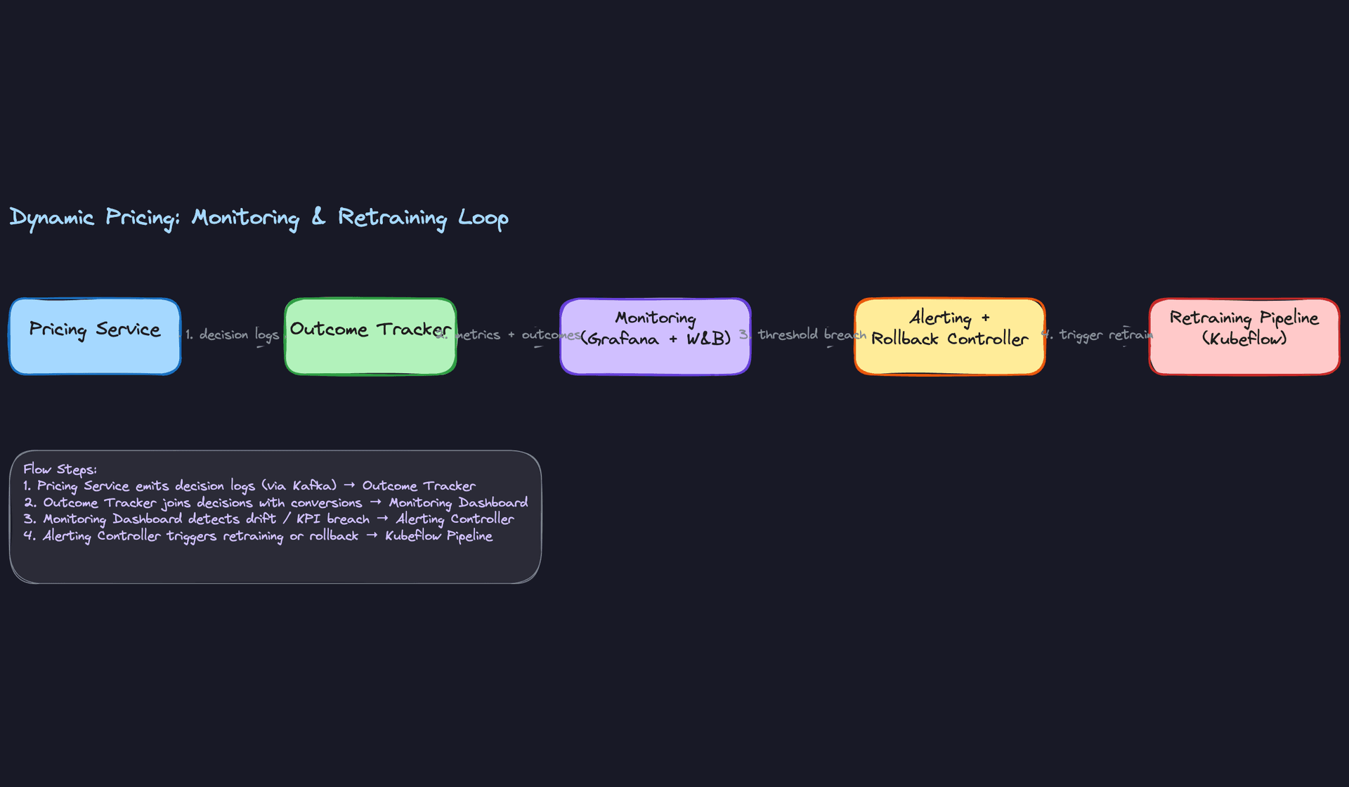
Closing the loop looks like this in practice:
- Monitoring detects that conversion rate in Chicago is down 12% over three days.
- On-call engineer checks the prediction distribution: model is pricing 8% higher than last week in that market.
- Feature audit shows competitor price index feed went stale two days ago, so the model is treating Chicago as having no competition.
- Fix the feed, retrain on the last 72 hours of clean data, run evaluation gates, promote to production.
- Add a monitor specifically for competitor feed staleness so this doesn't happen again.
That last step is the one most teams skip. Every incident should produce a new monitor.
Continuous Improvement
Retraining on a fixed daily schedule is fine as a starting point. For ride-hailing or food delivery, where supply/demand patterns shift with weather, events, and seasons, daily retraining on a 30-day rolling window keeps the model reasonably fresh. For more stable markets (e-commerce catalog pricing), weekly is often enough.
The more mature approach is drift-triggered retraining. Use a statistical test (Population Stability Index works well for tabular features) to compare the current input distribution against the training distribution. When PSI exceeds a threshold, trigger a retrain automatically via Kubeflow or Airflow. This is more responsive than a fixed schedule and avoids unnecessary retraining when nothing has changed.
Key insight: Drift-triggered retraining sounds sophisticated, but the hard part isn't the trigger. It's the evaluation gate. You need automated checks that a newly trained model is actually better before it goes to production. At minimum: offline holdout metrics must improve or stay flat, and a shadow deployment must show no regression on live traffic before you promote.
Once a model clears those gates, you still don't know if it moves the business metrics you actually care about. That's where A/B testing comes in. Split traffic by user or geographic market, route the control group to your current model and the treatment group to the candidate, and measure conversion rate, revenue per session, and cancellation rate over a statistically significant window. For pricing specifically, be careful about market-level interference: if you're testing surge pricing in a city, drivers and riders respond to the aggregate price signal, so a pure user-level split can produce misleading results. Geo-based holdouts (test in Seattle, hold out Portland as control) are cleaner for this reason.
A/B tests also give you something offline evaluation can't: evidence of how the model behaves under its own decisions. A model that looks great on historical data can still underperform in production because the historical data was generated by a different policy. Running a live experiment closes that gap.
When prioritizing model improvements, work in this order. First, fix data quality issues. A cleaner feature beats a fancier model almost every time. Second, add features that capture variance the model currently misses (nearby event data, real-time competitor feeds). Third, consider architecture changes (moving from XGBoost to a contextual bandit) only after the data pipeline is solid. Candidates who jump straight to "we should try RL" without addressing data quality first are skipping steps.
As the system matures, a few things change. Early on, you're mostly fighting data pipeline reliability and training-serving skew. Six months in, you're tuning the exploration-exploitation balance and worrying about fairness across markets. A year in, the biggest gains come from closing the feedback loop faster and personalizing at finer granularity. The model architecture often matters less than you'd expect. The monitoring and data infrastructure almost always matters more.
One risk that compounds over time: the model's own decisions corrupt the training data. If your model consistently underprices on Tuesday evenings, you'll never observe what would have happened at higher prices. Your training data develops blind spots that match your model's blind spots. Periodically inject random price exploration (with appropriate guardrails) to keep the training distribution honest. This is the argument for contextual bandits over pure supervised learning, and it's a point that lands well at the Staff level.
What is Expected at Each Level
Interviewers calibrate their expectations based on your level. The same question lands differently depending on whether you're a mid-level candidate who nails the basics or a staff engineer who proactively surfaces the problems nobody asked about.
Mid-Level
- Frame the business objective correctly before jumping to models. "We're maximizing revenue per session" is a better starting point than "we need to predict price."
- Propose XGBoost or LightGBM as your baseline regression model and justify it: interpretable, handles mixed feature types, trains fast on tabular data.
- Identify the core feature set: supply/demand ratio, hour of day, day of week, market zone. You don't need an exhaustive list, but you need the right instincts.
- Describe a basic A/B test to evaluate the model in production and know what a feature store is, even if you can't design one from scratch.
Senior
- Catch the training-serving skew problem without being prompted. Online features come from Redis; offline features come from batch snapshots. If those pipelines diverge, your model degrades silently.
- Explain counterfactual bias in your training data. You only observe outcomes at prices users accepted, so your model inherits the bias of your past pricing policy. Mention inverse propensity scoring or at least acknowledge the problem.
- Distinguish pre-computed price caches from real-time per-request inference, and articulate when each is appropriate. Ride-hailing needs sub-100ms; e-commerce catalog pricing can tolerate a batch job.
- Walk through a canary deployment: route 1-5% of traffic to the new model, define the rollback trigger (conversion drops more than X% week-over-week), and automate it.
Staff+
- Proactively raise feedback loop risk. High prices suppress demand, which reduces supply, which triggers even higher prices. A staff candidate names this, explains why it's dangerous, and proposes a monitoring strategy to catch runaway surge early.
- Drive the conversation toward exploration-exploitation tradeoffs. Supervised models trained on historical data can't discover better price points they've never tried. Contextual bandits or RL can, but they need guardrails to prevent the model from experimenting its way into a PR disaster.
- Address multi-market fairness and regulatory constraints without being asked. Price gouging laws, market-specific price sensitivity, and the ethics of personalized pricing are all in scope at this level.
- Describe how the system evolves over time: closed-loop retraining on fresh outcome data, automated evaluation gates before promotion, and cross-team dependencies (legal, finance, marketplace ops) that affect how fast you can ship model updates.
Key takeaway: Dynamic pricing is not a modeling problem with a deployment step bolted on. It's a closed-loop system where your model's outputs become tomorrow's training data. The candidates who stand out are the ones who design for that feedback loop from the start, not as an afterthought.
