Problem Formulation
Clarifying the ML Objective
ML framing: Given raw data and a declared task type, the platform must automatically produce a trained, validated model that optimizes a user-specified metric (e.g., AUC for classification, RMSE for regression) and deploy it as a callable endpoint.
The business goal here is deceptively simple: let teams ship ML models without needing a dedicated ML engineer for every project. The ML translation is harder. The platform has to solve a meta-learning problem, selecting the right model family, the right preprocessing strategy, and the right hyperparameters, without knowing in advance what the data looks like. It's not one ML task; it's a system that orchestrates many ML tasks automatically.
"Success" means different things depending on who you ask. A data scientist cares that the best model found is competitive with what they'd build by hand. A business user cares that the deployed model improves their KPI within a reasonable time budget. Your interviewer wants to see you hold both definitions at once, because a platform that finds a great model but takes 6 hours to do it will get abandoned.
Functional Requirements
Core Requirements
- Accept raw tabular, image, or text datasets and a declared task type (binary/multiclass classification, regression, ranking) as inputs; return a trained, deployed model endpoint.
- Run automated data validation and feature engineering before any search begins, including null checks, type inference, encoding selection, and train/val/test splitting.
- Execute hyperparameter search across a model zoo (LightGBM, XGBoost, MLP, and task-appropriate neural architectures) using at least one adaptive search strategy (Bayesian optimization or successive halving).
- Support one-click deployment of the best model to a versioned REST endpoint, with the full preprocessing pipeline bundled into the serving artifact.
- Trigger automated retraining when data drift or performance degradation is detected, seeding the new search from the prior best configuration.
Below the line (out of scope)
- Custom model architectures defined by the user (the platform operates over a fixed model zoo).
- Real-time streaming feature computation; the platform assumes batch-materialized features at training time.
- Multi-modal fusion tasks (e.g., combining image and tabular inputs in a single model).
Metrics
Offline metrics
The platform needs to track task-appropriate metrics per trial. For classification, AUC-ROC is the default because it's threshold-agnostic and handles class imbalance better than accuracy. For multiclass problems, you'd switch to macro-averaged F1 when classes are imbalanced or log-loss when you care about calibration. For regression, RMSE is the standard, but the platform should also surface MAE because RMSE penalizes outliers heavily and users need to know which error profile fits their use case. For ranking tasks, NDCG@K captures position-weighted relevance, which is what matters when the top results get most of the user attention.
Online metrics
Once deployed, the model's value is measured by downstream business outcomes. These vary by use case, but common ones include conversion rate lift (for propensity models), revenue per session (for pricing or recommendation models), and task completion rate (for any model embedded in a user workflow). The platform can't compute these directly, but it should expose hooks for users to pipe them back in as labeled feedback.
Guardrail metrics
- Inference latency: p99 must stay under the endpoint's declared SLA (default 200ms for synchronous REST).
- Prediction coverage: the fraction of requests that return a valid prediction rather than a fallback; should stay above 99.9%.
- Fairness: for classification tasks, the platform should surface demographic parity and equalized odds scores when sensitive columns are declared.
- Feature drift: PSI scores on input distributions, compared against the training baseline, tracked continuously post-deployment.
Tip: Always distinguish offline evaluation metrics from online business metrics. Interviewers want to see you understand that a model with great AUC can still fail in production. A common way to show this: point out that AUC measures ranking quality on a fixed test set, but online, the model's predictions change user behavior, which changes the data distribution. The test set goes stale.
Constraints & Scale
The platform needs to support 500 concurrent users, each potentially running multiple experiments. At 10,000 active experiments per day with an average of 50 trials each, that's 500,000 trial executions per day, roughly 6 trials per second sustained. Trial scheduling latency must stay under 5 seconds from config proposal to worker dispatch, or the HPO feedback loop slows down enough to hurt search quality.
Dataset sizes up to 100GB mean you can't load everything into a single worker's memory. Feature matrices need to be pre-computed and cached, and trial workers need to read from shared storage rather than re-running preprocessing on every trial.
| Metric | Estimate |
|---|---|
| Prediction QPS (deployed endpoints) | ~5,000 req/s across all active endpoints |
| Training data size | Up to 100GB per experiment |
| Model inference latency budget | p99 < 200ms (sync REST), throughput-optimized for batch |
| Feature freshness requirement | Batch-materialized; refreshed per retraining trigger |
| Active experiments per day | ~10,000 |
| Trial scheduling latency | < 5 seconds |
The hardest constraint is multi-tenant isolation. When a large team kicks off a neural architecture search with 500 trials, it can't starve out a small team's 10-trial tabular experiment. The scheduler needs per-tenant resource budgets enforced at the queue level, not just at the cluster level. This is a design decision you'll want to bring up proactively; interviewers at senior and staff levels will almost certainly ask about it.
Data Preparation
Before a single trial runs, your platform needs to answer a deceptively hard question: is this data actually ready to train on? Most AutoML failures aren't HPO failures. They're data failures that nobody caught.
Data Sources
The platform accepts data through three ingestion paths, and each one comes with different reliability guarantees.
Object storage (S3/GCS) is the most common path for batch datasets. Users point the platform at a bucket prefix, and the ingestion layer streams the files in. This works well for tabular CSVs and Parquet, but you need to handle schema inference on arrival because users rarely provide one upfront. Scan the first 10,000 rows, infer column types, and surface a preview before committing to a full ingest.
Database connectors let teams pull directly from Postgres, BigQuery, Snowflake, or Redshift via a JDBC/ODBC layer. Volume here can be large (tens of GBs per pull), and freshness depends entirely on the upstream write cadence. One thing to flag in your interview: connector-based ingestion introduces a live dependency. If the upstream table schema changes, your pipeline breaks silently unless you version the schema at ingest time.
REST upload API handles streaming uploads and smaller programmatic datasets. This is the path data scientists use when they're iterating quickly. Keep it simple: multipart upload, chunked transfer, checksum verification on completion.
Key insight: Schema inference is a convenience feature that becomes a correctness problem at scale. The platform should store the inferred schema as part of the dataset artifact, not just use it transiently. That schema becomes your contract for validation downstream.
For each ingestion path, the platform should record: source URI, ingest timestamp, row count, byte size, and the inferred schema. These four fields are what make debugging possible six months later.
Label Generation
This is where most candidates wave their hands and move on. Don't.
Labels in an AutoML platform come from the user, and the platform needs to handle three fundamentally different cases.
Explicit labels are the easy case: a CSV column the user designates as the target. Classification targets, regression targets, ranking scores. The platform validates that the column exists, checks for nulls, and for classification counts the class distribution.
Implicit labels are trickier. A user might upload a clickstream table and say "predict conversion." The platform needs to join event sequences into a single training row, derive the binary label from a downstream event (purchase = 1, no purchase within 7 days = 0), and handle the observation window carefully.
Human annotation is the hardest operationally. If a user uploads raw text or images and expects the platform to help them label it, that's a separate annotation workflow. For an AutoML platform design, it's reasonable to scope this out and say: "We assume labels arrive pre-annotated."
Warning: Label leakage is one of the most common ML system design mistakes. Always clarify the temporal boundary between features and labels. If your label is "did the user churn in the next 30 days" and one of your features is "account status at end of month," you've leaked the future into your features. The platform should enforce a label_horizon parameter that timestamps the feature snapshot cutoff.Label quality issues the platform should surface automatically:
- Noise: For classification, flag if label agreement rate is low (relevant when labels come from multiple annotators or heuristic rules).
- Delayed feedback: If labels are derived from downstream events, some rows will have incomplete labels at training time. The platform should warn when the dataset's most recent rows fall within the feedback delay window.
- Class imbalance: Flag when the minority class is below 5% of the dataset. This isn't a blocker, but the platform should note it and apply stratified sampling automatically.
def validate_labels(df: pd.DataFrame, label_col: str, task_type: str) -> LabelReport:
    report = LabelReport()

    # Null check
    null_rate = df[label_col].isna().mean()
    report.null_rate = null_rate
    if null_rate > 0.05:
        report.warnings.append(f"Label column has {null_rate:.1%} null rate")

    if task_type == "classification":
        class_dist = df[label_col].value_counts(normalize=True)
        minority_rate = class_dist.min()
        report.class_distribution = class_dist.to_dict()
        if minority_rate < 0.05:
            report.warnings.append(
                f"Minority class is {minority_rate:.1%} of data. "
                "Stratified sampling will be applied."
            )

    return report
Data Processing and Splits
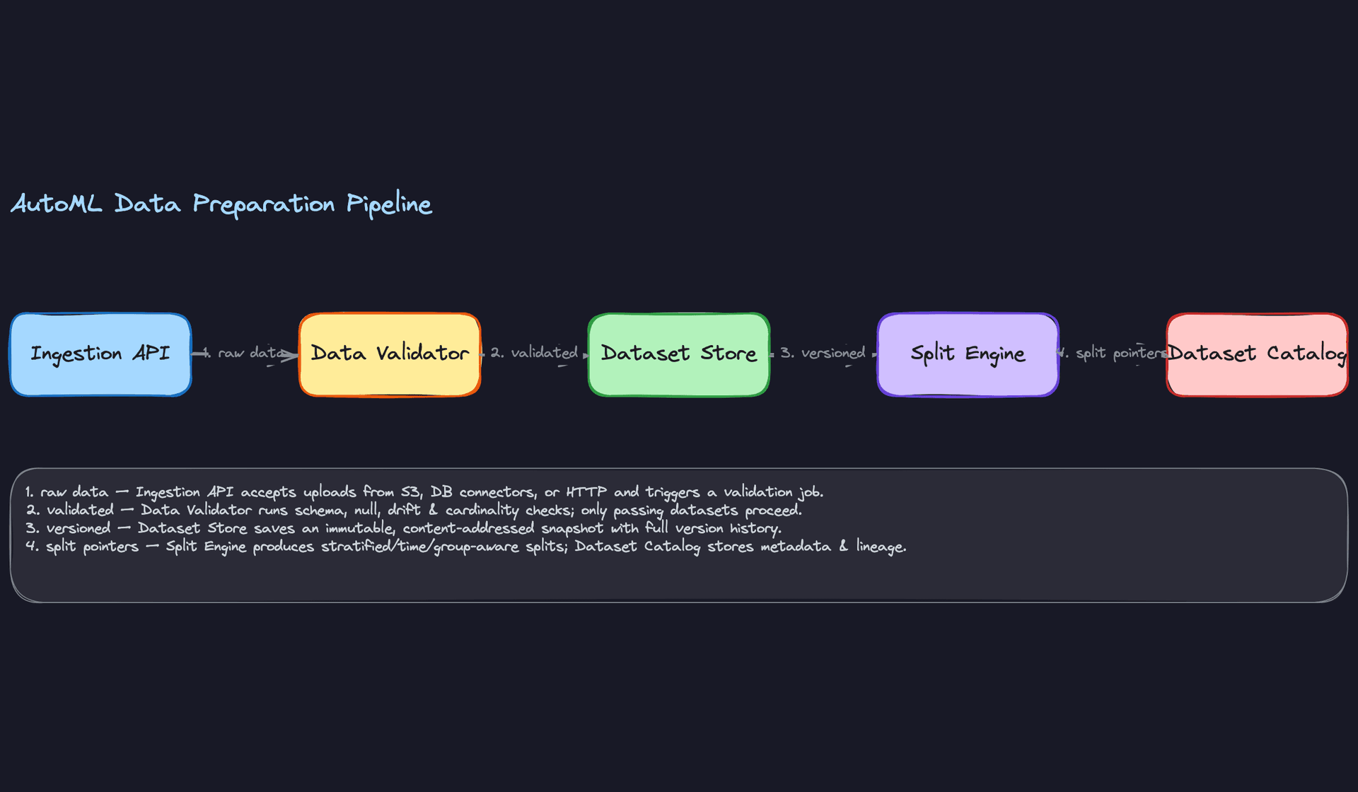
Automated validation runs before any pipeline proceeds. Think of it as a gate, not a suggestion. The platform runs four checks in sequence:
- Null rate check: Any column exceeding a configurable threshold (default 40%) gets flagged. The platform can either drop the column or impute, depending on user config.
- Type consistency: If the inferred schema says a column is numeric but 15% of values are non-parseable strings, that's a data quality issue, not a type inference issue.
- Cardinality check for categoricals: A categorical column with 500,000 unique values in a 600,000-row dataset is almost certainly a leaky ID column. Flag it.
- Distribution drift against a reference split: If the user is uploading a new dataset to retrain an existing model, the platform computes PSI (Population Stability Index) against the training baseline. PSI > 0.2 triggers a warning before the experiment starts.
All four checks must pass before the experiment scheduler sees the dataset. Fail fast here, not three hours into a training run.
Deduplication happens next. The platform hashes each row and drops exact duplicates. For image or text datasets, near-duplicate detection (MinHash LSH) is worth offering as an option, though it's expensive at scale. In your interview, it's fine to say: "For v1, we do exact deduplication. Near-duplicate detection is a follow-up."
Splitting strategy is where the platform earns its keep. Random splits are almost always wrong for production ML, and the platform should make the right choice by default based on task type.
For classification and regression on non-temporal data, stratified splits preserve class distribution across train/val/test. For forecasting and any time-series task, the platform enforces time-based splits: train on the past, validate on a more recent window, test on the most recent window. This isn't optional. A random split on time-series data leaks future information into training, and your model will look great in validation and fail immediately in production.
For datasets with natural groups (users, sessions, geographic regions), group-aware splits ensure that all rows from a given group land in exactly one split. This prevents the model from memorizing group-level patterns and calling it generalization.
def create_splits(
    df: pd.DataFrame,
    strategy: Literal["stratified", "time_based", "group_aware"],
    label_col: str,
    time_col: str = None,
    group_col: str = None,
    val_ratio: float = 0.15,
    test_ratio: float = 0.15,
) -> DatasetSplits:

    if strategy == "time_based":
        assert time_col is not None, "time_col required for time_based strategy"
        df_sorted = df.sort_values(time_col)
        n = len(df_sorted)
        train_end = int(n * (1 - val_ratio - test_ratio))
        val_end = int(n * (1 - test_ratio))
        return DatasetSplits(
            train=df_sorted.iloc[:train_end],
            val=df_sorted.iloc[train_end:val_end],
            test=df_sorted.iloc[val_end:],
        )

    elif strategy == "group_aware":
        assert group_col is not None
        groups = df[group_col].unique()
        np.random.shuffle(groups)
        n_groups = len(groups)
        train_groups = groups[:int(n_groups * (1 - val_ratio - test_ratio))]
        val_groups = groups[len(train_groups):int(n_groups * (1 - test_ratio))]
        test_groups = groups[int(n_groups * (1 - test_ratio)):]
        return DatasetSplits(
            train=df[df[group_col].isin(train_groups)],
            val=df[df[group_col].isin(val_groups)],
            test=df[df[group_col].isin(test_groups)],
        )

    # Default: stratified
    ...
Dataset Versioning and Lineage
Every dataset snapshot the platform stores is content-addressed. The platform computes a SHA-256 hash of the file contents and uses that as the storage key. Two users uploading identical files get the same key, which means zero duplication in object storage. More importantly, every experiment record stores a pointer to this immutable hash, not a mutable file path.
CREATE TABLE dataset_versions (
    id            UUID PRIMARY KEY DEFAULT gen_random_uuid(),
    content_hash  VARCHAR(64) NOT NULL UNIQUE,  -- SHA-256 of raw bytes
    source_uri    TEXT NOT NULL,                 -- original upload location
    row_count     BIGINT NOT NULL,
    byte_size     BIGINT NOT NULL,
    schema        JSONB NOT NULL,               -- inferred column types
    split_config  JSONB NOT NULL,               -- strategy + ratios used
    created_at    TIMESTAMP NOT NULL DEFAULT now(),
    created_by    UUID NOT NULL REFERENCES users(id)
);

CREATE TABLE experiment_dataset_links (
    experiment_id  UUID NOT NULL REFERENCES experiments(id),
    dataset_id     UUID NOT NULL REFERENCES dataset_versions(id),
    split_role     VARCHAR(10) NOT NULL,  -- 'train', 'val', 'test'
    PRIMARY KEY (experiment_id, split_role)
);
The dataset catalog is what makes this auditable. When a model underperforms in production, you can trace back through the experiment to the exact dataset version, including its schema, split config, and validation report. Without this, you're debugging blind.
Common mistake: Candidates often design the model registry carefully but treat datasets as ephemeral. In a production AutoML platform, dataset versioning is just as important as model versioning. If you can't reproduce a training run exactly, you can't debug it, and you can't satisfy compliance requirements in regulated industries.
The lineage graph the platform maintains connects: trigger event (if retrain) → experiment → dataset version → split config → model artifact. Every node in that chain is immutable and addressable by ID. That's what "reproducibility" actually means in practice, not just saving the model weights.
Feature Engineering
The AutoML platform can't know in advance whether it's looking at a column of zip codes, Unix timestamps, or product descriptions. So before any model search begins, it needs to figure out what it's working with and how to turn it into numbers a model can actually use.
Feature Categories
The platform organizes every column it encounters into one of four types, each with its own transformation strategy.
Numeric features are the simplest case, but "simplest" doesn't mean trivial. A raw dollar amount and a user's age both look numeric, but they have wildly different distributions. The platform selects a scaling strategy per column: standard scaling for roughly Gaussian distributions, min-max for bounded ranges, and log-transform for heavy-tailed signals like revenue or click counts.
Concrete examples: - purchase_amount (float): log-scaled, then standardized - account_age_days (int): min-max normalized to [0, 1] - session_page_views (int): log-transform to compress outliers - product_price (float): quantile normalization to handle price skew
Categorical features need encoding, and the right encoding depends on cardinality. Low-cardinality columns (under ~20 unique values) get one-hot encoded. High-cardinality columns, like product IDs or zip codes, get target encoding or learned embeddings, because one-hot at 50,000 categories is just a sparse disaster.
Concrete examples: - device_type (string, 5 values): one-hot encoded - product_category (string, 200 values): target encoding against the label - user_country (string, 180 values): embedding lookup (dim=16) - payment_method (string, 8 values): one-hot encoded
Datetime features are where a lot of AutoML systems fall flat. Feeding a raw Unix timestamp into a model is almost useless. The platform decomposes datetime columns into cyclical components using sine/cosine encoding so the model understands that 11:59 PM and 12:01 AM are close together.
Concrete examples: - event_timestamp: decomposed into hour_sin, hour_cos, day_of_week_sin, day_of_week_cos - signup_date: converted to days_since_signup (numeric) - last_purchase_date: converted to recency_days relative to event time
Free text features get either TF-IDF (fast, interpretable, works well for short structured text like product titles) or a sentence embedding via a pretrained model like sentence-transformers. The platform picks TF-IDF by default and upgrades to embeddings if the column has high average token count or if the user specifies it.
Concrete examples: - product_title (short text): TF-IDF, top 500 terms - user_review (long text): sentence-transformer embedding, 384 dims - search_query (short text): TF-IDF or embedding depending on vocab diversity
Missing Value Handling
Real-world datasets are never clean. Before any transformation runs, the platform profiles each column for missingness and applies an imputation strategy based on column type, missing rate, and distributional shape.
For numeric columns, the default is median imputation (more resistant to outliers than mean), but the platform also adds a binary indicator flag, is_missing_<column_name>, alongside the imputed value. That flag matters: missingness itself is often predictive. A user with no last_purchase_date is probably a new user, and that signal shouldn't be silently erased by filling in the median.
# Imputation with missingness indicator
from sklearn.impute import SimpleImputer
import numpy as np

class NumericImputer:
    def fit(self, X):
        self.median_ = np.nanmedian(X, axis=0)
        return self

    def transform(self, X):
        indicator = np.isnan(X).astype(int)          # 1 where value was missing
        X_imputed = np.where(np.isnan(X), self.median_, X)
        return np.hstack([X_imputed, indicator])     # append indicator columns
For categorical columns, the platform imputes with a constant "__MISSING__" token rather than the mode. This keeps the missingness visible to the model as a distinct category, which is almost always better than pretending the most common value appeared.
High-missingness columns (over 70% missing) get flagged for review. The platform doesn't silently drop them, but it does surface a warning in the experiment report. Sometimes a column is 80% null because it only applies to a subset of users, and that subset is exactly who you care about.
Key insight: K-NN imputation is more accurate than median/mode but runs in O(n²) time. For datasets over a few million rows, it's not practical without approximation. The platform defaults to statistical imputation and offers K-NN as an opt-in override for smaller datasets where accuracy matters more than speed.
Automated Feature Generation
This is where the "Auto" in AutoML earns its name. Beyond transforming existing columns, the platform actively generates new features that the user never explicitly defined.
Interaction terms capture relationships between pairs of features. A model might learn that account_age_days and purchase_count_30d individually are weak signals, but their ratio (purchase_rate) is strong. The platform generates pairwise products and ratios for numeric columns, then uses a fast correlation filter to keep only the ones that add signal above a threshold.
# Automated interaction term generation
from itertools import combinations
import pandas as pd

def generate_interactions(df: pd.DataFrame, numeric_cols: list) -> pd.DataFrame:
    new_features = {}
    for col_a, col_b in combinations(numeric_cols, 2):
        new_features[f"{col_a}_x_{col_b}"] = df[col_a] * df[col_b]
        # Ratio only where denominator is safe
        safe_denom = df[col_b].replace(0, float("nan"))
        new_features[f"{col_a}_div_{col_b}"] = df[col_a] / safe_denom
    return pd.DataFrame(new_features)
Polynomial features are generated selectively, not blindly. Applying degree-2 expansion to 100 numeric columns produces 5,000 new columns, most of which are noise. The platform limits polynomial expansion to columns that show a nonlinear relationship with the target (detected via a mutual information test) and caps the degree at 2 for anything going into a linear model.
Datetime-derived aggregates are another category the platform generates automatically. If the dataset has both a signup_date and an event_timestamp, the platform computes days_since_signup without being asked. If there are multiple timestamp columns, it generates all pairwise deltas.
Common mistake: Candidates sometimes propose generating all possible features and letting the model sort it out. That works for tree-based models that do implicit selection, but it will destroy a linear model's performance and bloat training time. Feature generation and feature selection have to be designed together.
Automated Feature Selection
Generated features need to be pruned. The platform runs a selection stage after generation, before any model trials begin, using a tiered approach.
The first pass is statistical: columns with near-zero variance get dropped immediately. A column that's the same value for 99% of rows contributes nothing. This is cheap and catches obvious garbage fast.
The second pass uses mutual information scores between each feature and the target label. Features below a configurable threshold get removed. This is fast enough to run on the full dataset and catches irrelevant features that happen to have high variance.
from sklearn.feature_selection import mutual_info_classif
import numpy as np

def select_by_mutual_info(X, y, threshold=0.01):
    scores = mutual_info_classif(X, y, random_state=42)
    selected = np.where(scores >= threshold)[0]
    return selected, scores
The third pass is model-based. The platform trains a lightweight gradient boosted tree (a fast LightGBM run with early stopping) and uses feature importances to rank the remaining columns. The bottom quartile gets dropped. This catches features that look correlated with the target in isolation but add nothing once other features are present.
For high-dimensional datasets, the platform also offers PCA as an optional dimensionality reduction step, particularly useful when the input includes dense embeddings (384-dim sentence vectors, for example). PCA runs after imputation and scaling, before model search, and the number of components is chosen to retain 95% of explained variance by default.
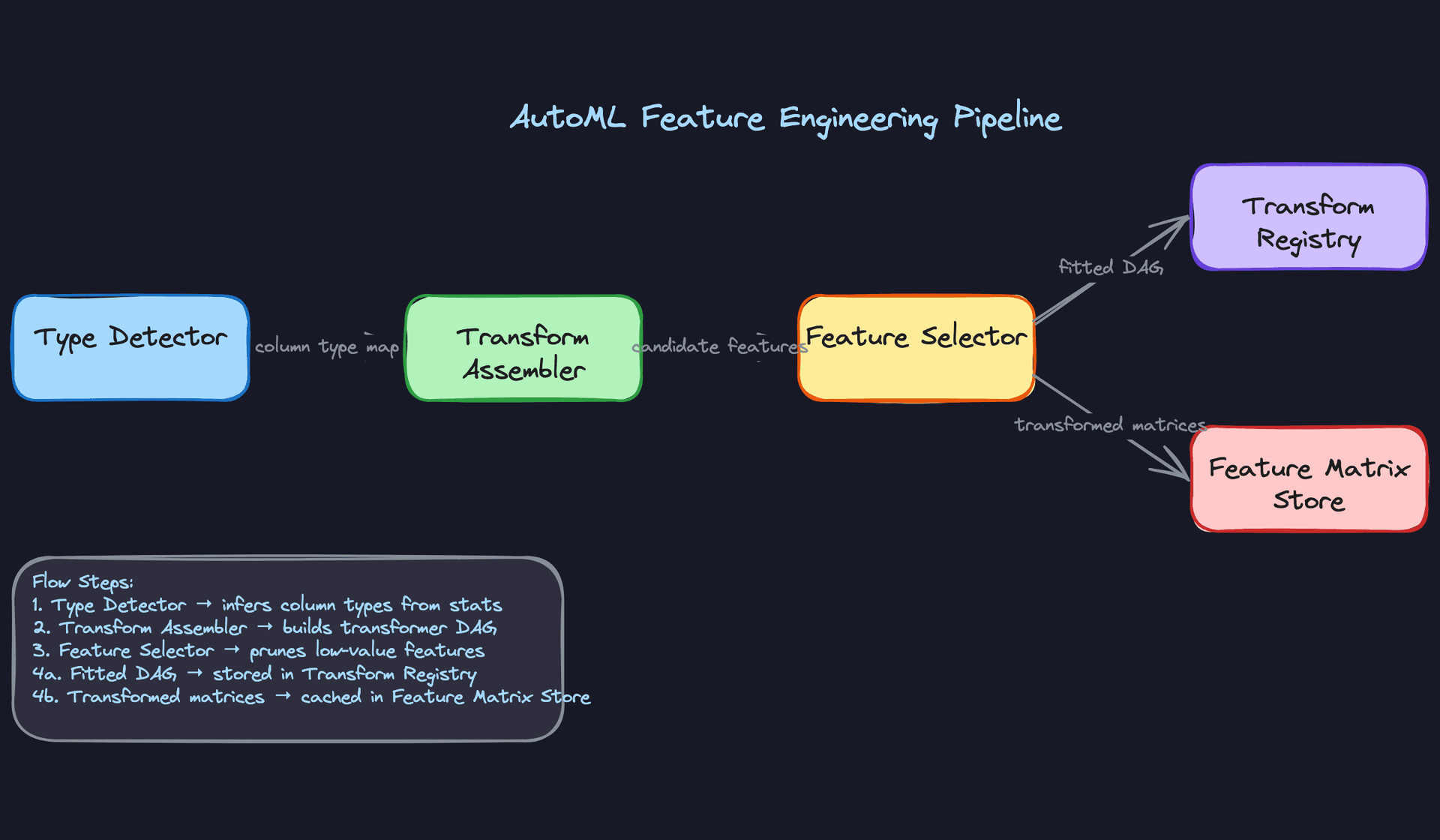
Interview tip: When an interviewer asks how your AutoML platform handles feature engineering, don't just describe transformations. Walk through the full pipeline: type detection, imputation, generation, selection, then transformation. That sequence signals you understand the problem end to end, not just the happy path.
Feature Computation
The platform assembles a transformation DAG automatically based on detected types. Each node in the DAG is a stateless, serializable transformer. Stateless matters here: the fitted parameters (mean, std, vocabulary, embedding weights) live in the node's config, not in mutable state, so the entire DAG can be serialized to disk and reloaded identically at serving time.
Batch features are computed offline on a schedule using Spark or SQL jobs. A typical example: a user's 30-day purchase count, computed nightly from the transactions table and written to the offline feature store as a Parquet partition. The pipeline looks like this:
# Spark job: compute 30-day user purchase aggregates
from pyspark.sql import functions as F

user_features = (
    transactions
    .filter(F.col("event_date") >= F.date_sub(F.current_date(), 30))
    .groupBy("user_id")
    .agg(
        F.count("*").alias("purchase_count_30d"),
        F.sum("amount").alias("purchase_value_30d"),
        F.countDistinct("product_category").alias("category_diversity_30d"),
    )
)

user_features.write.mode("overwrite").parquet("s3://feature-store/user_features/date=2024-01-15/")
These features land in the offline store and get joined to training data at experiment time. Freshness is typically 24 hours, which is fine for signals that change slowly.
Near-real-time features require a streaming pipeline. Items a user viewed in the last 10 minutes, for example, can't wait for a nightly batch job. The platform routes clickstream events through Kafka, processes them with Flink, and writes aggregates to the online store with a short TTL.
# Flink job: sliding window aggregation of recent views
from pyflink.datastream import StreamExecutionEnvironment
from pyflink.datastream.window import SlidingEventTimeWindows
from pyflink.common.time import Time

env = StreamExecutionEnvironment.get_execution_environment()

view_stream = (
    env.from_source(kafka_source, watermark_strategy, "clickstream")
    .key_by(lambda e: e["user_id"])
    .window(SlidingEventTimeWindows.of(Time.minutes(10), Time.minutes(1)))
    .aggregate(ViewCountAggregator())
)

view_stream.add_sink(redis_sink)  # writes user_id -> view_count_10m to Redis
Flink's event-time windowing is important here. Processing-time windows will silently produce wrong results when events arrive out of order, which they always do.
Real-time features are computed at request time, during the serving call itself. The canonical example is embedding the current search query. You can't precompute this because the query is unknown until the user types it.
# Called inside the serving handler, per request
def compute_realtime_features(request: dict) -> dict:
    query_text = request.get("search_query", "")
    query_embedding = embedding_model.encode(query_text)  # ~5ms on CPU, <1ms on GPU

    return {
        "query_embedding": query_embedding.tolist(),
        "query_length": len(query_text.split()),
        "has_filters": int(bool(request.get("filters"))),
    }
Keep real-time computation cheap. Anything over ~10ms starts eating into your p99 latency budget. If a real-time feature requires a heavy model, cache it aggressively or move it to near-real-time.
Feature Store Architecture
The platform uses a dual-store architecture. The offline store (Parquet on S3/GCS, queryable via Hive or Spark) holds the full historical feature table used to build training datasets. The online store (Redis or DynamoDB) holds the latest feature values for each entity, served at low latency during inference.
Key insight: The most common failure mode in ML systems is training-serving skew. Features computed differently in batch training vs. online serving will silently degrade your model. Always design for consistency.
The way you prevent skew is by making the transformation logic the single source of truth. The platform serializes the fitted transformer DAG alongside the model artifact. At serving time, the same DAG runs on incoming request data before the model sees it.
# Serialized transformer DAG stored with every model artifact
import joblib

# Training time: fit and serialize
pipeline = FeatureTransformPipeline(column_specs)
pipeline.fit(X_train)
joblib.dump(pipeline, "artifacts/transformer_dag_v3.pkl")

# Serving time: load and apply identically
pipeline = joblib.load("artifacts/transformer_dag_v3.pkl")
features = pipeline.transform(raw_request_features)
prediction = model.predict(features)
The online store lookup happens before the transformer DAG runs. The serving handler fetches precomputed batch and near-real-time features from Redis using the entity key (user ID, item ID), computes any real-time features inline, concatenates everything, then passes the full feature vector through the DAG.
One thing that trips up candidates: the offline store and online store will have different feature values for the same entity at the same moment. That's expected. The offline store is a historical log; the online store is a point-in-time snapshot. What must be consistent is the transformation logic applied to those values, not the values themselves.
User Overrides
The automated path handles the common case, but data scientists often know things the platform doesn't. Maybe a column that looks numeric is actually an ordinal code and shouldn't be standardized. Maybe a custom tokenizer is needed for domain-specific text.
The platform exposes a config layer for this:
# experiment_config.yaml
feature_overrides:
  product_code:
    type: categorical          # override: platform detected numeric
    encoding: target_encoding
  user_review:
    type: text
    encoder: custom
    encoder_path: s3://my-bucket/domain-tokenizer-v2.pkl
  internal_flag:
    exclude: true              # drop this column entirely
  purchase_amount:
    imputation: knn            # override default median imputation
    imputation_k: 5
  account_tenure:
    generate_interactions: false  # suppress interaction generation for this column
Overrides slot into the DAG at the column level without touching the rest of the automated pipeline. The platform validates the override config at experiment submission time, not at trial start, so you find out immediately if you've pointed to a nonexistent encoder path rather than 40 minutes into a training run.
Common mistake: Candidates often propose feature engineering as a one-time preprocessing step that runs before the experiment. In a real AutoML platform, the transformer DAG is part of the model artifact. If you separate them, you will have skew in production. The DAG ships with the model, always.
Model Selection & Training
The core of any AutoML platform is the search loop: given a dataset and a task type, find the best model without requiring the user to know what "best" even means. Getting this right requires thinking carefully about what you search over, how you search, and when you stop.
Model Architecture
Start With a Baseline
Before any search begins, the platform trains a fixed baseline: logistic regression for classification, ridge regression for regression. No tuning, no feature selection magic. Just fit and score.
This matters for two reasons. First, it gives you a sanity check. If your fancy LightGBM ensemble can't beat logistic regression on a given dataset, something is wrong with your pipeline, not the data. Second, it sets a floor that the HPO search has to clear before you'd ever promote a more complex model to production.
Interview tip: Mentioning baselines signals maturity. Interviewers know that candidates who skip straight to XGBoost have probably debugged fewer production incidents than those who start simple.
The Model Zoo
The platform maintains a curated model zoo rather than an open-ended search space. For tabular data, that means LightGBM, XGBoost, logistic/ridge regression, and a shallow MLP. For image inputs, a small CNN backbone (ResNet-18 or EfficientNet-B0). For text, a fine-tuned DistilBERT or a TF-IDF plus gradient boosting pipeline depending on dataset size.
Each model in the zoo ships with a prior over its hyperparameter space. LightGBM's prior covers num_leaves (32-512, log-uniform), learning_rate (1e-3 to 0.3, log-uniform), min_child_samples (5-100), and regularization terms. These priors aren't arbitrary; they're calibrated from thousands of prior experiments using meta-learning, so the search starts in a region that tends to work rather than sampling blindly from the full space.
The input/output contract is fixed per task type:
# Classification trial contract
class TrialContract:
    # Inputs
    X_train: np.ndarray       # shape (n_samples, n_features), float32
    y_train: np.ndarray       # shape (n_samples,), int for classification
    X_val: np.ndarray
    y_val: np.ndarray
    task_type: str            # "classification" | "regression" | "ranking"

    # Outputs
    val_score: float          # primary metric (AUC, RMSE, NDCG)
    loss_curve: List[float]   # per-epoch val loss, used for early stopping
    wall_time_seconds: float
    model_artifact_path: str  # versioned artifact path, e.g. s3://models/{experiment_id}/{trial_id}/v{version}/
    prediction_latency_p99_ms: float
    feature_importances: Dict[str, float]  # feature name -> importance score (e.g. SHAP or gain)
    shap_values_sample_path: str           # path to SHAP values computed on a held-out sample; NULL if not supported
Every trial, regardless of model type, writes to this same schema. The scheduler doesn't need to know whether it's evaluating XGBoost or a transformer; it just reads val_score and loss_curve.
The model_artifact_path always points to a versioned, immutable location. Overwriting artifacts in place is not allowed. This is what makes experiment reproducibility tractable: you can always re-load the exact model that produced a given trial's scores, months after the experiment ran.
The feature_importances and shap_values_sample_path fields are populated during training, not as a post-hoc step. For tree models, gain-based importance is essentially free. For neural models, the platform computes SHAP on a 1,000-row sample using a background dataset. These outputs feed directly into the error analysis UI and the fairness slice reports, so debugging a bad model doesn't require re-running anything.
Training Pipeline
Three HPO Strategies, Chosen by Context
Random search is the baseline HPO strategy and it's more competitive than it sounds. Because trials are independent, you can run hundreds in parallel across your worker pool with zero coordination overhead. For small datasets where each trial completes in under a minute, random search with 200 trials often matches Bayesian optimization in wall-clock time while being far simpler to operate.
Bayesian optimization via TPE (Tree-structured Parzen Estimator, implemented through Optuna) is the default for medium-to-large experiments. TPE fits two density estimators: one over configurations that performed well, one over configurations that didn't. The next config is sampled to maximize the ratio of the first to the second. In practice, this means the search converges on good regions of the hyperparameter space in 30-50 trials rather than 150-200.
The catch with Bayesian optimization is that it's sequential by design. Each new suggestion depends on all prior results, so you can't fully parallelize. The platform handles this with a batch suggestion mode: Optuna proposes a batch of K configs simultaneously using a "constant liar" strategy, where pending trials are treated as if they returned the current best score. It's an approximation, but it lets you run 8-16 parallel workers without stalling the search.
Common mistake: Candidates describe Bayesian optimization as strictly better than random search. It isn't. For high-dimensional search spaces (>20 hyperparameters), TPE's surrogate model degrades and random search often wins. Know the tradeoff.
Successive halving and Hyperband are the right tools when trial duration varies widely across model types. The idea is simple: run all trials for one epoch, eliminate the bottom half by validation score, double the budget for survivors, repeat. A neural architecture search that would cost 500 GPU-hours with full training costs roughly 50 with Hyperband because you kill bad configs early.
The platform uses Hyperband as the default for any experiment that includes neural models in the search space, and falls back to TPE for pure tabular searches where trial durations are short and uniform.
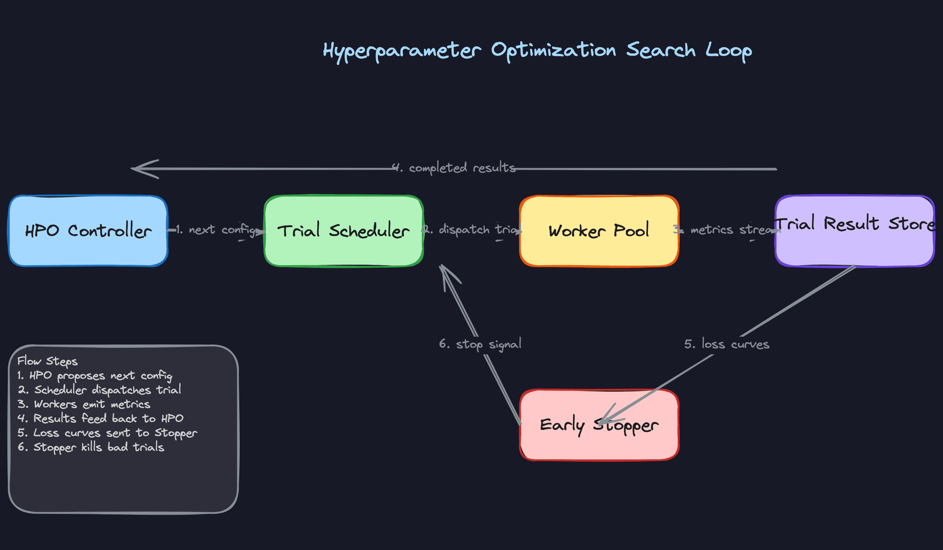
Trial Scheduling and Multi-Tenant Fairness
A central scheduler maintains a priority queue of pending trials across all active experiments. When a worker pod becomes available, the scheduler pops the highest-priority trial and dispatches it.
Priority is a function of two things: experiment age (older experiments get a small boost to prevent starvation) and per-tenant resource budgets. Each tenant gets a configurable CPU-hour and GPU-hour budget per day. The scheduler tracks running consumption and deprioritizes trials from tenants who are close to their limit. This prevents one team running a 10,000-trial neural search from starving out everyone else on the cluster.
# Simplified scheduling priority score
def compute_priority(trial: Trial, tenant: Tenant) -> float:
    budget_remaining_fraction = (
        tenant.daily_gpu_budget_hours - tenant.consumed_gpu_hours
    ) / tenant.daily_gpu_budget_hours

    age_boost = min(trial.wait_time_seconds / 3600, 2.0)  # cap at 2.0

    return budget_remaining_fraction * trial.experiment_priority + age_boost
Workers are heterogeneous: CPU pods for tabular models, GPU pods for neural trials. The scheduler matches trial type to resource type at dispatch time, so a LightGBM trial never sits waiting for a GPU to free up.
One question interviewers sometimes push on: does the scheduler support preemption, or only priority-ordered dispatch? The platform supports soft preemption for neural trials. If a high-priority trial is waiting and all GPU pods are occupied by lower-priority work, the scheduler can signal the lowest-priority running trial to checkpoint and yield. The trial saves its current epoch state, the pod is released, and the preempted trial re-queues with its checkpoint path attached so it resumes rather than restarts. Preemption is opt-in per experiment because it adds checkpoint overhead, and it's disabled by default for short tabular trials where the overhead isn't worth it.
The Trial Result Store
Every worker streams metrics back to a time-series store (InfluxDB or a similar append-optimized store) as training progresses, not just at the end. This serves two purposes.
The HPO controller reads completed trial results to update its surrogate model and propose the next batch of configs. The early stopper reads in-progress loss curves and compares them against the median curve of all trials at the same epoch. If a trial is tracking below the 20th percentile at 30% of its budget, it gets killed. This is the mechanism that makes Hyperband work in practice.
The UI reads from the same store to show live loss curves and a live leaderboard. Users can watch trials converge in real time rather than waiting for a batch result at the end.
Worker failures are an operational reality. When a worker pod dies mid-trial, the scheduler detects the missing heartbeat after a configurable timeout (default: 90 seconds) and marks the trial as FAILED. Partial metric streams are retained in the time-series store for debugging but are excluded from surrogate model updates and leaderboard ranking. The trial is automatically re-queued once, with the same hyperparameter config, so a transient infrastructure failure doesn't silently drop a potentially good configuration. If the retry also fails, the trial is marked DEAD and flagged in the experiment report. A high DEAD rate is itself a signal worth surfacing: it usually means the config is requesting more memory than the pod can provide, not that the underlying model is bad.
Training Infrastructure
Tabular trials run on CPU pods with 4-8 cores and 32GB RAM. A LightGBM trial on a 10GB dataset typically completes in 2-10 minutes. Neural trials (MLP, CNN, transformer fine-tuning) run on single-GPU pods (A10G or T4 depending on model size), with multi-GPU reserved for large foundation model fine-tuning, which is outside the default search space.
For distributed training within a single trial, the platform uses PyTorch DDP for neural models when the dataset exceeds GPU memory. This is rare in the default search space but supported for custom model types.
Retraining frequency is driven by the monitoring layer (covered in the next section), but the default cadence for scheduled retraining is weekly for most production models, with a full search rather than incremental fine-tuning. Incremental fine-tuning sounds appealing but it accumulates bias toward recent data distributions and makes reproducibility harder. Full retraining from a versioned dataset snapshot is the safer default.
Offline Evaluation
Metrics That Connect to Business Outcomes
The platform surfaces a primary metric per task type: AUC-ROC for binary classification, RMSE for regression, NDCG for ranking. But AUC alone will get you in trouble. A model with 0.92 AUC can still be badly miscalibrated, meaning its predicted probabilities don't reflect actual event rates. For any model that feeds into a decision threshold (fraud scoring, churn prediction, loan approval), calibration matters as much as discrimination.
The platform runs a calibration check on every candidate model using the Brier score and reliability diagrams. A model that's well-calibrated but slightly lower AUC than the leader is often the better production choice.
Interview tip: Interviewers want to see that you evaluate models rigorously before deploying. "It has good AUC" is not enough. Discuss calibration, fairness slices, and failure modes.
Fairness slices are evaluated automatically for classification tasks. The platform computes AUC and false positive rate across any categorical columns the user flags as sensitive (age bucket, region, device type). A model that achieves 0.91 AUC overall but 0.78 AUC on a minority slice fails the promotion gate, regardless of its leaderboard position.
Evaluation Methodology
The holdout test set is set aside at dataset ingestion time and never touched during search. This is non-negotiable. Candidates who describe using the validation set for final model selection and the test set for reporting are describing a leaky evaluation setup.
For time-series and forecasting tasks, the platform uses walk-forward backtesting: train on data up to time T, evaluate on T to T+window, slide forward, repeat. This catches models that look great on a random split but fail because they've implicitly seen future data through feature leakage.
Cross-validation is reserved for small datasets (under 50k rows) where a single holdout split would be too noisy to trust. The platform uses 5-fold stratified CV in that regime and averages scores across folds before ranking trials.
Baseline Comparisons and Error Analysis
Every experiment report shows three numbers side by side: the logistic regression baseline, the best single model from search, and the ensemble. If the gap between baseline and best single model is small (under 2% AUC), the platform flags it as a "data-limited" experiment and recommends collecting more labeled data rather than continuing to search.
Error analysis is the part most candidates skip. The platform buckets validation errors by input feature quantiles and surfaces the slices with the highest error concentration. If your model's worst predictions cluster in the top decile of a particular numeric feature, that's a signal that the feature needs a different transformation or that the model is extrapolating outside its training distribution. The SHAP values stored in shap_values_sample_path feed directly into this view, so you can see not just where the model fails but which features are driving those failures.
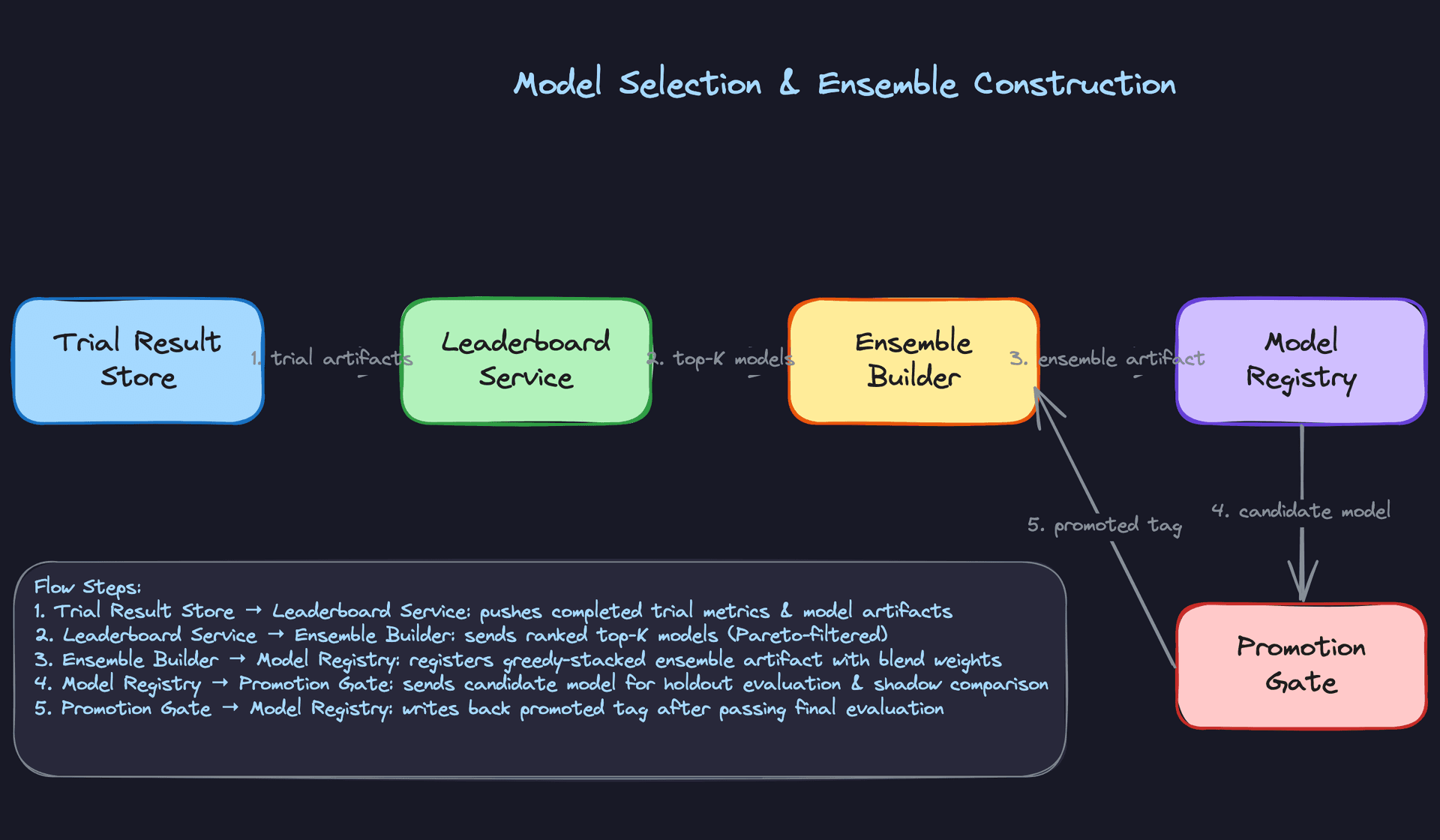
Ensemble and Final Model Selection
After search completes, the platform takes the top-K trials (default K=10) and runs a greedy ensemble stacking step. Starting with the single best model, it greedily adds models that improve validation score when blended, using held-out validation predictions to fit blend weights. Typically 3-5 models contribute meaningfully; beyond that, marginal gains disappear and you're adding serving complexity for nothing.
The final selection isn't always the ensemble. The platform exposes a Pareto front view with three axes: validation score, p99 prediction latency, and model memory footprint. Latency and memory are related but distinct constraints. A single LightGBM model might be 5ms p99 and 80MB in memory. An ensemble of five models might be 40ms p99 and 600MB. For a latency-sensitive fraud API, the latency axis dominates. For deployment to an edge device with 256MB of available RAM, memory footprint is the binding constraint and the ensemble is simply not an option regardless of its AUC advantage.
Surfacing all three axes lets the user make an informed tradeoff rather than having the platform make it for them. A 0.3% AUC improvement is worth different things in different deployment contexts, and the platform shouldn't pretend otherwise.
Inference & Serving
Most AutoML platforms nail the training side and then bolt on a Flask app as an afterthought. That's where they die in production. The serving layer is where your design needs to be just as deliberate as the HPO loop.
Serving Architecture
Online vs. Batch: Choosing the Right Mode
AutoML serves two very different user personas. A fraud detection team needs sub-100ms predictions on individual transactions as they arrive. A marketing team wants churn scores for 10 million customers every Sunday night. These are fundamentally different problems, and your platform needs to handle both without forcing users to choose an architecture.
The decision rule is straightforward: if the consumer needs a prediction before they can proceed (a user waiting for a page to load, a payment waiting to be approved), that's online inference. If the consumer can wait minutes or hours and will process predictions in bulk, that's batch. For an AutoML platform, you'll see both constantly, so both paths need to be first-class citizens.
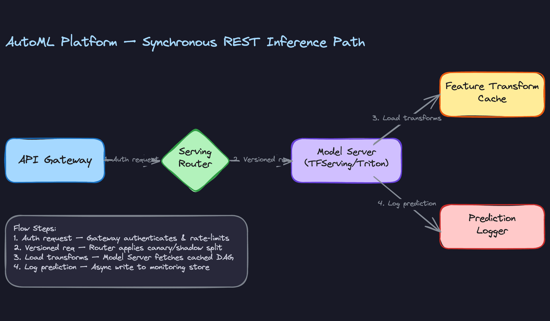
The synchronous path is the more latency-sensitive one. A request comes in through the API gateway, gets authenticated and rate-limited, then the serving router decides which model version handles it based on the current traffic split config. The model server runs the preprocessing DAG (loaded from the feature transform cache) and then the forward pass, and the prediction gets logged asynchronously so it doesn't add to tail latency.
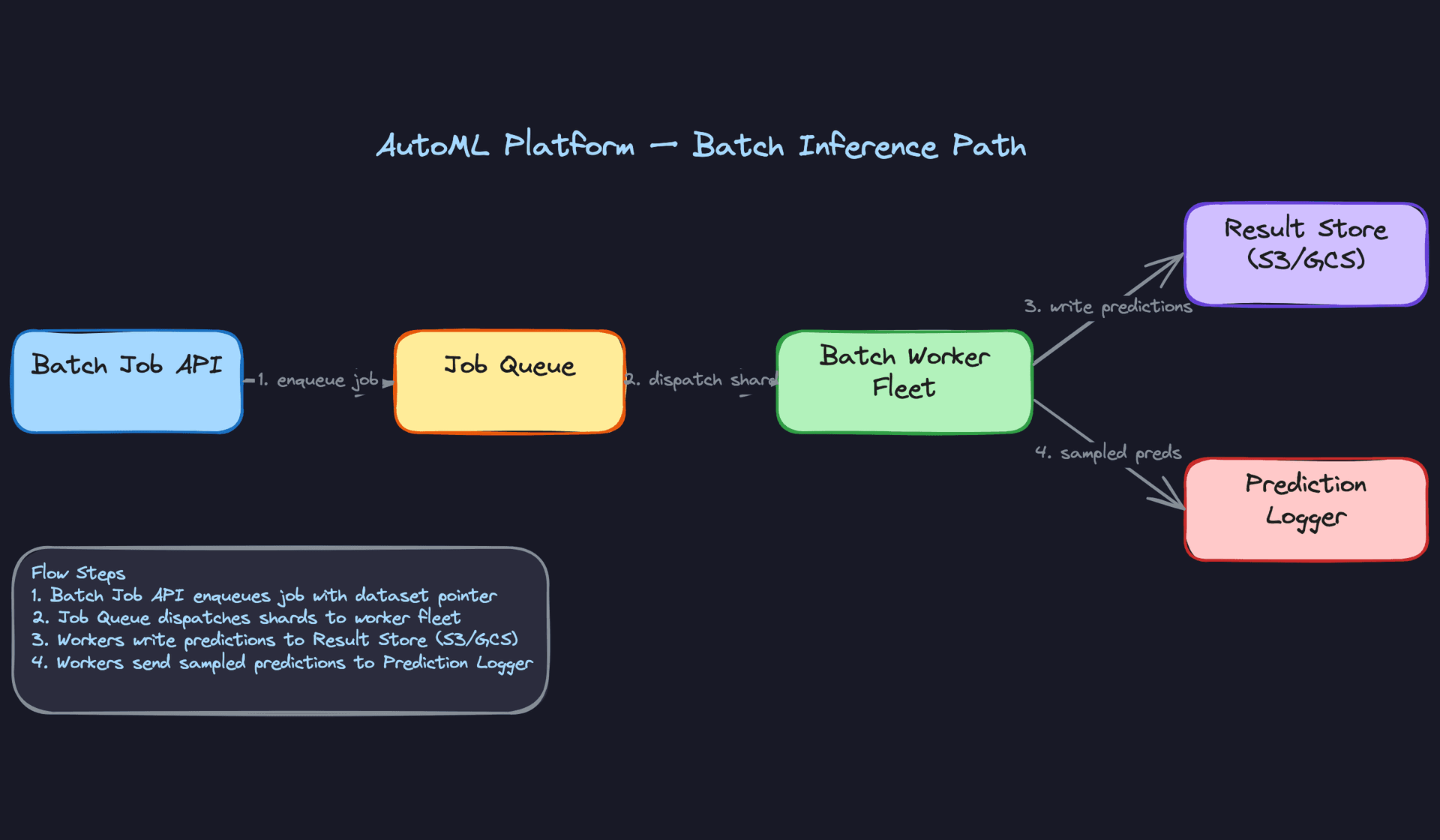
Batch inference is simpler to reason about but has its own failure modes. The job gets enqueued, a worker fleet pulls dataset shards from object storage, applies the same transformer DAG, runs inference, and writes partitioned Parquet files back to S3 or GCS. The key thing to get right here is idempotency: if a worker crashes mid-shard, it should be safe to re-run without producing duplicate predictions.
Model Serving Infrastructure
For tabular models (LightGBM, XGBoost, sklearn pipelines), a custom Python service with FastAPI and a process pool is often the right call. These models are CPU-bound and lightweight; Triton adds complexity without much benefit.
For neural models (MLPs, CNNs, transformers), Triton Inference Server is the right choice. It handles multi-framework model loading (TensorFlow SavedModel, ONNX, PyTorch TorchScript), dynamic batching, and GPU memory management out of the box. TFServing works if your model zoo is TF-only, but Triton's framework agnosticism fits AutoML better since your search space spans multiple frameworks.
Interview tip: If the interviewer asks why not just use TFServing, the answer is framework lock-in. AutoML platforms need to serve whatever model won the search, and that might be an XGBoost tree one day and a PyTorch transformer the next.
Request Flow End-to-End
Here's the full latency budget for a synchronous prediction:
- API gateway auth + routing: 2-5ms. JWT validation, rate limit check, route to the right model endpoint.
- Feature transform: 5-20ms. The fitted transformer DAG is cached in memory on the model server. First request after a cold start pays the deserialization cost (50-200ms); subsequent requests hit the in-process cache.
- Model inference: 1-50ms for tabular models; 10-200ms for neural models depending on size and whether you're on GPU.
- Post-processing: 1-5ms. Threshold application, label decoding, confidence calibration.
- Async prediction logging: fire-and-forget, doesn't block the response.
Total p99 target: under 100ms for tabular, under 300ms for neural. If you're blowing past those, the feature transform step is usually the culprit.
Optimization
Model Optimization Before Serving
The model that wins the HPO search isn't necessarily the model you should serve. Before deployment, the platform should run a post-training optimization pass.
For neural models, quantization (INT8 or FP16) typically cuts inference latency by 2-4x with less than 1% accuracy drop on most tabular and NLP tasks. ONNX export plus ONNX Runtime gives you hardware-optimized execution for CPU serving without touching the model architecture. For very large models, knowledge distillation into a smaller student model is worth the effort if you have strict latency SLAs.
For tree-based models, the main optimization is prediction caching. If your use case has repeated inputs (same user, same features within a short window), an LRU cache keyed on the feature vector hash can eliminate a large fraction of actual model calls.
Common mistake: Candidates propose quantization without mentioning the accuracy regression check. Always validate the optimized model against the original on the holdout set before swapping it in.
Batching Strategies
Dynamic batching is the single biggest throughput lever for GPU-served models. Instead of running one forward pass per request, the model server accumulates requests for a short window (1-5ms) and processes them as a single batch. Triton handles this natively. The tradeoff is added latency for low-traffic periods, so you need a max-wait timeout to bound the worst case.
For CPU-served tabular models, batching matters less. The overhead of accumulating a batch often exceeds the compute savings. Serve requests individually and scale horizontally instead.
GPU vs. CPU Serving
GPU serving makes sense when your model has enough compute density to saturate the GPU. A 3-layer MLP on tabular data doesn't; a BERT-based text classifier does. The rule of thumb: if your model has fewer than 10 million parameters and your batch size is under 64, CPU serving is cheaper and simpler to operate.
For the AutoML platform, the default should be CPU serving for tabular models and GPU serving for neural models, with the serving bundle metadata encoding which hardware class the model requires. The trial scheduler already knows this from the training run, so the deployment system can inherit it automatically.
Fallback Strategies
Every model endpoint needs a fallback. When the model server is unavailable or exceeds a latency threshold, the platform should fall back to the previous promoted model version (which is kept warm). If that's also unavailable, fall back to a simple heuristic: the training set's majority class for classification, the training set mean for regression.
Don't return an error to the caller if you can help it. A degraded prediction is almost always better than a 503.
Online Evaluation and A/B Testing
Traffic Splitting and Experiment Assignment
A/B testing ML models is different from A/B testing UI changes. The assignment unit matters. For user-level models, assign by user ID so the same user always sees the same model version. For transaction-level models, you can assign by request ID. Consistent hashing on the assignment key keeps the split stable across restarts.
The serving router reads the experiment config from a control plane (a simple key-value store works fine) and routes traffic accordingly. A typical ramp looks like: 5% to the challenger, 95% to the champion. The router stamps each prediction log with the model version and experiment ID so you can split metrics downstream.
Online Metrics and Statistical Methodology
For classification, track AUC, precision, recall, and calibration error on the live label stream (once labels arrive via the feedback loop). For regression, track MAE and RMSE. For ranking, track NDCG or MRR.
Use a sequential testing framework (like mSPRT or always-valid confidence intervals) rather than fixed-horizon t-tests. With fixed-horizon tests, peeking at results early inflates your false positive rate. Sequential tests let you stop early when you have enough evidence without paying a statistical penalty.
Key insight: The deployment pipeline is where most ML projects fail in practice. A model that can't be safely deployed and rolled back is a model that won't ship.
Set your minimum detectable effect before the experiment starts. For most AutoML use cases, a 1-2% improvement in the primary metric is worth shipping. Anything smaller is noise at the scale of a typical team's traffic.
Ramp-Up and Rollback
Ramp in stages: 1% → 5% → 20% → 50% → 100%. Pause between stages and check for metric regressions. Automate the pause: the platform should halt the ramp if error rate exceeds a threshold or if the primary metric degrades by more than X% relative to the champion.
Rollback should be a single API call that instantly pins traffic back to the previous champion. The previous two model versions stay hot (loaded in memory on the serving fleet) so rollback doesn't require a cold start. Target: traffic fully back on the champion within 30 seconds of triggering rollback.
Interleaving for Ranking Systems
If your AutoML platform supports ranking tasks (search, recommendations), interleaving is worth implementing. Instead of splitting users between two models, interleave results from both models for every user and track which model's results get clicked. Interleaving detects differences with 10-100x less traffic than A/B testing because every user is exposed to both models simultaneously.
The implementation is more complex (you need to track which model contributed each result and de-duplicate overlapping results), but for ranking use cases it's the right call when you need fast decisions.
Deployment Pipeline
Validation Gates Before Promotion
A model doesn't get deployed just because it won the HPO search. It has to pass a gauntlet first.
The promotion gate runs three checks. First, holdout evaluation: the model is scored on the test split (which was never touched during training or validation). If it underperforms the currently-serving model by more than a configurable threshold, it's blocked. Second, latency profiling: the serving bundle is loaded into a staging environment and hit with a synthetic load test. If p99 latency exceeds the SLA, it's blocked. Third, schema validation: the model's expected input schema is compared against the current production data schema. A mismatch here means training-serving skew is guaranteed.
def run_promotion_gate(
    candidate_model_id: str,
    champion_model_id: str,
    holdout_dataset_id: str,
    latency_sla_ms: float = 100.0,
    regression_threshold: float = 0.02,  # 2% relative degradation
) -> PromotionResult:
    candidate_score = evaluate_on_holdout(candidate_model_id, holdout_dataset_id)
    champion_score  = evaluate_on_holdout(champion_model_id, holdout_dataset_id)

    relative_delta = (candidate_score - champion_score) / champion_score
    if relative_delta < -regression_threshold:
        return PromotionResult.BLOCKED, f"Regression: {relative_delta:.2%}"

    p99_latency = run_load_test(candidate_model_id, duration_s=60)
    if p99_latency > latency_sla_ms:
        return PromotionResult.BLOCKED, f"Latency SLA breach: {p99_latency:.1f}ms"

    schema_ok = validate_input_schema(candidate_model_id)
    if not schema_ok:
        return PromotionResult.BLOCKED, "Input schema mismatch"

    return PromotionResult.APPROVED, "All gates passed"
Canary Deployment
Once the promotion gate passes, the model enters canary. It receives 5-10% of live traffic while the champion handles the rest. The platform monitors error rate, latency, and (when labels are available quickly enough) prediction quality in real time.
Canary runs for a configurable window, typically 24-48 hours. If no regressions are detected, the ramp continues automatically. If a regression is detected, the canary is killed and traffic snaps back to the champion.
Shadow Scoring
Shadow mode runs the challenger on 100% of traffic but discards its predictions. Users only see the champion's output. This is the safest way to validate a new model because it eliminates sampling variance: you're comparing both models on identical inputs.
Shadow scoring is especially valuable when the challenger uses a different feature set or preprocessing pipeline. You can catch training-serving skew before it ever affects a real user. The cost is double the compute during the shadow period, which is acceptable for high-stakes deployments.
Interview tip: Interviewers love asking "how do you know the new model is safe to deploy?" Shadow scoring is the right answer for high-stakes systems. Canary is the right answer when compute cost is a constraint. Know when to use each.
Rollback Triggers
Automated rollback fires on any of these conditions:
- Error rate on the challenger exceeds 1% (vs. champion baseline)
- p99 latency increases by more than 50% relative to the champion
- Primary metric degrades by more than 2% relative during canary
- A manual trigger from an on-call engineer
The previous two model versions stay hot on the serving fleet at all times. Rollback is a config change to the serving router, not a redeployment. That's the difference between a 30-second recovery and a 10-minute one.
Monitoring & Iteration
A model that works on launch day is not a model that works six months later. Data distributions shift, user behavior changes, upstream pipelines quietly break. The platform needs to catch all of this automatically, because no one is watching dashboards at 3am.
Production Monitoring
Data drift is your earliest warning signal, and it fires before your accuracy metrics even move. For every deployed model, the platform stores a statistical baseline of the training feature distribution. At inference time, a background sampler collects input features and runs Population Stability Index (PSI) and Kolmogorov-Smirnov tests against that baseline on a rolling window. PSI above 0.2 on any feature triggers a warning; above 0.25 triggers a retraining event.
Schema violations are a separate, harder failure. A feature that was always a float suddenly arrives as a string. A categorical column gains a new cardinality value the encoder has never seen. The platform validates incoming feature vectors against the schema snapshot frozen at training time, and any mismatch gets flagged before the model ever runs. Silent type coercions are worse than loud failures.
Model monitoring splits into two layers depending on whether you have labels.
Without labels, you watch prediction drift: the distribution of model outputs over time. A classifier that was outputting 60/40 positive/negative last week but is now outputting 90/10 this week has probably seen something it wasn't trained on. You can detect this with no ground truth at all.
With labels, you compute live accuracy, AUC, or whatever metric the experiment was optimized for. The platform joins incoming ground-truth labels (via the label ingestion API described below) with logged predictions and recomputes performance metrics continuously. This is the gold standard signal, but it's often delayed.
System monitoring is table stakes but worth being explicit about in an interview. The platform tracks p50/p95/p99 inference latency, request throughput, error rates per endpoint, and GPU utilization across the serving fleet. These feed into standard alerting (PagerDuty, OpsGenie) and are separate from the ML-specific signals above. An interviewer who asks "how do you know the system is healthy?" wants to hear both layers.
Common mistake: Candidates describe ML monitoring but forget system monitoring entirely. Interviewers at senior+ levels notice this gap immediately. Latency spikes and GPU saturation are model health issues too.
Alerting thresholds should be tiered. Soft thresholds send a Slack notification to the model owner. Hard thresholds trigger automated retraining. Critical thresholds (e.g., error rate above 5%) trigger automatic rollback to the previous model version. The platform exposes these thresholds as configurable per-model settings, because a fraud detection model and a product recommendation model have very different risk tolerances.
SHAP values add explainability on top of the raw drift scores. The platform computes SHAP on a sample of recent predictions and surfaces feature importance in the UI, so a user can see not just "drift was detected" but "the account_age feature is driving 60% of the distribution shift." That distinction matters for diagnosis: is this a data pipeline bug or a genuine population change?
Feedback Loops
The hardest part of closing the loop is that labels are almost never immediate.
For click-through rate models, you might have a label within seconds. For churn prediction, the label arrives 30 days after the prediction. For fraud detection, it can take weeks of investigation. The platform handles this with a label ingestion API that accepts ground-truth labels asynchronously, keyed to the original prediction ID. The join happens in a time-windowed table: predictions are held in a buffer, and as labels arrive they get matched and flushed into the accuracy computation.
# Label join logic (simplified)
def join_labels_to_predictions(
    prediction_log: pd.DataFrame,
    label_batch: pd.DataFrame,
    max_delay_days: int = 30
) -> pd.DataFrame:
    merged = prediction_log.merge(
        label_batch,
        on="prediction_id",
        how="left"
    )
    # Drop predictions older than max_delay_days that never received a label.
    # These are unresolvable: the label window has closed and we exclude them
    # from accuracy computation rather than treating them as negatives.
    cutoff = pd.Timestamp.now() - pd.Timedelta(days=max_delay_days)
    expired_unlabeled = (merged["predicted_at"] < cutoff) & merged["label"].isna()
    merged = merged[~expired_unlabeled]
    return merged[merged["label"].notna()]
When labels are delayed, you have two options. First, use proxy signals: clicks, conversions, user reports, or downstream business metrics that correlate with model quality. These aren't perfect but they're available now. Second, accept partial accuracy estimates computed on the fraction of predictions that have resolved labels so far, and weight them appropriately. The platform surfaces both.
User feedback beyond labels matters too. If downstream systems expose explicit signals (a user flags a recommendation as irrelevant, a reviewer overrides a fraud decision), those flow through the same label ingestion API. The platform treats them as soft labels with configurable confidence weights.
The full loop looks like this:
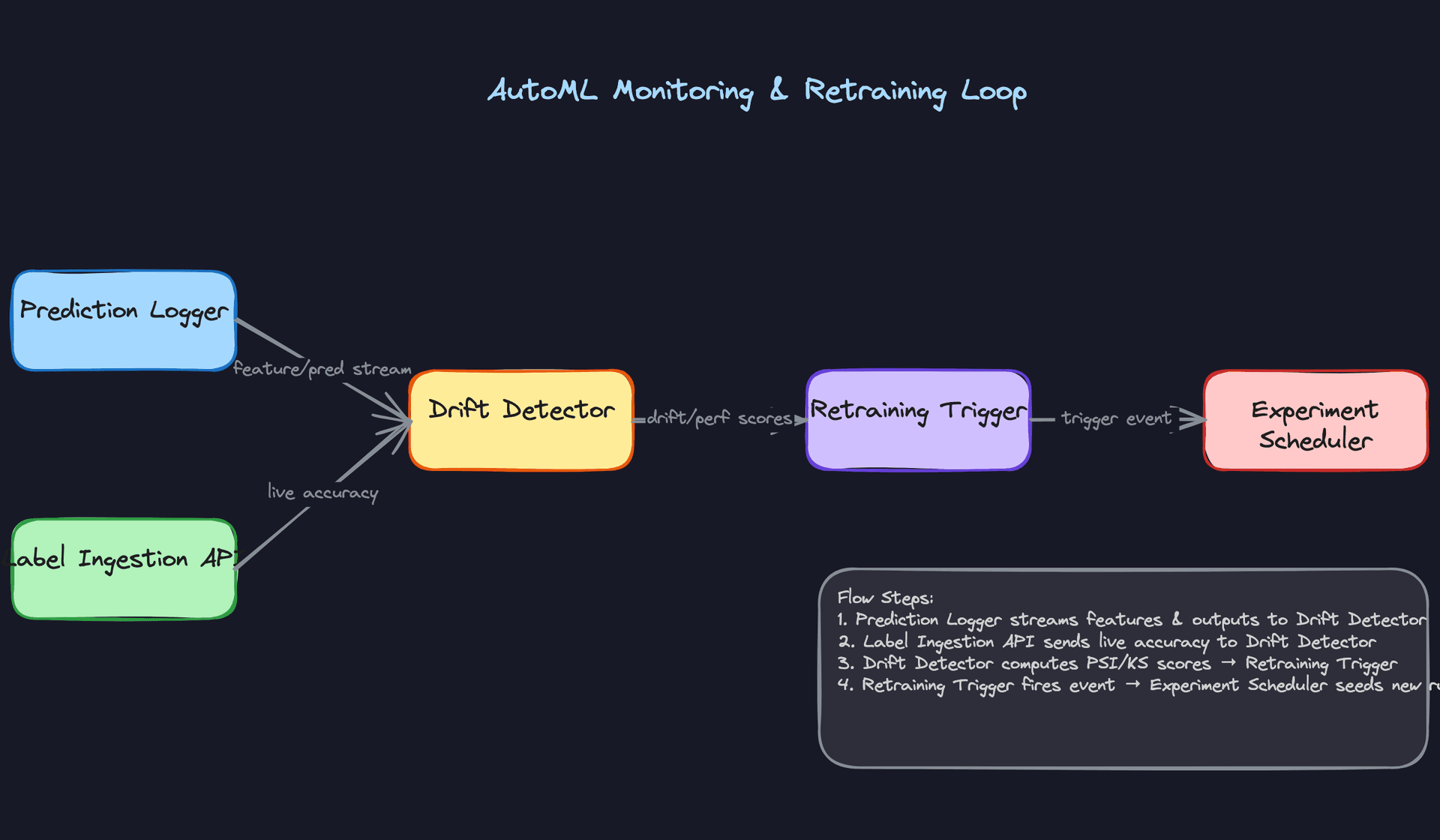
Monitoring alert fires. The platform's rules engine identifies which signal breached threshold and tags the trigger reason. A new experiment is automatically created, seeded with the parent experiment's best hyperparameter configuration as warm-start priors for the HPO search. The new experiment runs against a refreshed dataset that includes the recent data window. After search completes, the promoted model goes through canary deployment before replacing the current version. Every step links back to the trigger event in the lineage graph, so you can audit exactly why a model changed.
Tip: Staff-level candidates distinguish themselves by discussing how the system improves over time, not just how it works at launch.
Continuous Improvement
Scheduled retraining and drift-triggered retraining solve different problems. Scheduled retraining (weekly, monthly) is appropriate when your data distribution is relatively stable but you want to incorporate new training examples over time. Drift-triggered retraining is appropriate when your distribution is volatile and you can't predict when the model will degrade. The platform supports both, and the right answer for a given model depends on its domain.
One thing to get right: triggered retraining should not run the full search from scratch every time. That's expensive and slow. The warm-start approach uses the parent experiment's best config as the center of the new search space, with a narrower exploration radius. This cuts search time significantly while still allowing the model to adapt if the optimal architecture has shifted.
Prioritizing improvements as the system matures follows a rough hierarchy. Data quality issues first: garbage in, garbage out, and no amount of architecture search fixes a broken feature pipeline. Feature additions second: new signals that weren't available at launch often have more impact than tuning existing ones. Architecture changes last: switching from LightGBM to a transformer is expensive to validate and usually only justified when you've exhausted the simpler levers.
As the platform accumulates experiments across many datasets and tasks, a meta-learning layer becomes viable. The platform can learn which model families and hyperparameter ranges tend to perform well on datasets with similar statistical properties (row count, feature cardinality, class imbalance ratio). New experiments start with priors informed by this history rather than generic defaults. Google's Vizier and AutoSklearn both implement versions of this. At Staff level, proposing this as a long-term evolution of the platform is the kind of answer that signals you're thinking about the system as a product, not just a pipeline.
One more thing that changes as the system matures: governance requirements. Regulated industries (finance, healthcare) often can't deploy ensemble models because they need single-model interpretability for audits. The platform needs a configuration flag that disables the ensemble step and enforces single-model selection, with SHAP-based explanations attached to every prediction. Building this as a first-class feature rather than an afterthought is what separates a platform that works in a startup from one that works in an enterprise.
What is Expected at Each Level
Interviewers calibrate their expectations based on seniority, and AutoML is a topic where the gap between levels is unusually wide. A mid-level answer that stops at "run a grid search and deploy the best model" is fine. A staff-level answer that stops there is a red flag.
Mid-Level
- Walk through the full pipeline end-to-end: data ingestion, automated feature engineering, HPO using random or Bayesian search, and deployment as a REST endpoint. You don't need to invent novel algorithms; you need to show you understand how the pieces connect.
- Name the core failure modes unprompted. Training-serving skew (fitting transformers on the full dataset before splitting), missing early stopping (burning compute on clearly bad trials), and no dataset versioning (making experiments unreproducible) are the three the interviewer is listening for.
- Demonstrate basic HPO intuition. Know that random search is a legitimate baseline, not a cop-out, and that Bayesian optimization with TPE makes sense when trials are expensive and you have a meaningful budget (50+ trials).
- Show you understand why automation needs guardrails. Data validation before any pipeline proceeds, stratified splits for imbalanced classification, and schema checks on new data uploads are the kinds of details that signal production awareness.
Senior
- Go deep on HPO strategy tradeoffs. Hyperband and successive halving shine when trial cost varies widely (seconds to hours); Bayesian optimization wins when the search space is small and each trial is expensive. Know when to use which, and say so explicitly.
- Design the trial scheduler for multi-tenant fairness. A shared worker pool without resource budgets per tenant means one team's 500-trial neural architecture search starves everyone else. Propose fair-share scheduling, per-experiment resource caps, and priority queues.
- Articulate the canary and shadow deployment flow with specifics. Shadow mode runs both the old and new model on 100% of traffic but only serves the old model's predictions; canary actually splits live traffic. Conflating them is a common senior-level slip.
- Propose a drift-triggered retraining loop with concrete thresholds. "Monitor for drift" is not enough. Say PSI > 0.2 on key input features triggers a warm-started re-experiment, and that the new experiment inherits the parent's best hyperparameter config as a prior to cut search time.
Staff+
- Reason about the platform as a product serving two very different users. Data scientists want to override search spaces, pin encodings, and inspect every trial. Business users want to upload a CSV and get a deployed model in an hour. A staff candidate proposes a layered abstraction: full automation by default, with a config layer that exposes control without breaking the automated path.
- Propose meta-learning across experiments. After the platform has run thousands of experiments, it has a signal: which model families and hyperparameter ranges tend to win on datasets with similar statistical profiles (row count, feature cardinality, class imbalance). A search space warm-start layer that transfers these priors across datasets can cut median experiment cost by 30-50%.
- Address cost efficiency as a first-class design concern. Spot instances for trial workers with checkpointing, early stopping budgets enforced at the scheduler level, and tiered storage for trial artifacts (hot for recent, cold for archived) are the kinds of decisions that separate a platform that works from one that a company can actually afford to run at scale.
- Handle regulated industry constraints on the ensemble step. Greedy stacking produces a black-box blend that a bank or healthcare company cannot ship. A staff candidate flags this and proposes a Pareto-front selection mode that surfaces the single best interpretable model (logistic regression, shallow tree) alongside SHAP explanations, with the ensemble available only when interpretability requirements are relaxed.
Key takeaway: AutoML is not just about automating model training. It is about building a system that is reproducible, fair across tenants, safe to deploy, and self-improving over time. The candidates who stand out are the ones who treat automation as a product decision, not just an engineering shortcut.
