Problem Formulation
Most personalization systems fail not because the model is wrong, but because the team never agreed on what "right" means. Before you write a single line of training code, you need to nail down what the model is actually predicting, what signals it learns from, and what latency envelope it has to live inside.
Start by asking the interviewer: what are we personalizing? Feed items, ads, search results, and product recommendations are all ranking problems at heart, but they have very different label distributions, latency requirements, and business constraints. A feed ranking system optimizing for dwell time is a different beast from an ad auction optimizing for expected revenue. Get this on the table early.
Clarifying the ML Objective
ML framing: Given a user and their current context, score and rank a set of candidate items by predicted engagement probability so the most relevant items appear first.
The business goal is engagement: keep users on the platform, drive clicks, purchases, or watch time. The ML translation is a ranking problem over a candidate set. You're predicting some form of user-item affinity, typically a probability of click or conversion, and using that score to order items.
"Success" means different things depending on who you ask. The product team cares about CTR, session length, and revenue. The ML team cares about AUC and NDCG on a held-out evaluation set. These are correlated but not identical. A model that perfectly predicts clickbait titles will score well offline and tank long-term retention. Make sure you say this out loud in the interview; it signals that you think about the full product loop, not just the loss function.
The core ML task is typically framed as pointwise ranking: predict a score per user-item pair, then sort. This is simpler to train than pairwise or listwise approaches and scales more easily to millions of candidates. At the retrieval stage, you're doing approximate nearest-neighbor search over embeddings, not scoring every item individually. The two-stage architecture (retrieval then ranking) is the standard answer for any catalog larger than a few thousand items.
Functional Requirements
Core Requirements:
- The system must return a ranked list of N items (typically 10-100) for a given user and context within a p99 latency of 100ms end-to-end.
- The ranking model takes as input: user features (recent interaction history, long-term preferences), item features (content embeddings, popularity, freshness), and context features (device, time of day, session position).
- User context must reflect interactions from at least the last few minutes. A user who just clicked three sports articles should see more sports content on the next page load, not results computed from yesterday's batch job.
- The system must handle cold-start users (no interaction history) by falling back to content-based or popularity-based signals rather than returning an error or a random list.
- The output is a ranked list with scores, not a single item. Downstream business logic (diversity filters, sponsored content injection) will post-process the list before it reaches the user.
Below the line (out of scope):
- Real-time model retraining or online learning during serving. We'll retrain on a scheduled cadence (daily or weekly), not update weights per request.
- Multi-objective ranking that jointly optimizes for engagement and revenue in a single model. That's a separate problem with its own complexity.
- Personalized search query understanding. We're ranking a pre-defined candidate set, not doing query rewriting or semantic search.
Metrics
Offline metrics tell you how well the model learned from historical data. They're necessary but not sufficient.
- AUC-ROC measures the model's ability to separate clicked from non-clicked items across all possible thresholds. It's threshold-agnostic and handles class imbalance well, which matters here because click rates are typically 1-5%.
- NDCG@K (Normalized Discounted Cumulative Gain) is the right metric when you care about ranking quality, not just binary classification. It rewards putting the most relevant items at the top of the list and penalizes burying them at position 8 vs. position 2. Use K=10 or K=20 to match your actual display window.
- MRR (Mean Reciprocal Rank) is useful if you're optimizing for the first relevant result, common in search-adjacent personalization tasks.
Online metrics are what actually matter for the business:
- CTR (click-through rate) is the most direct signal that the ranked list is relevant. It's noisy and gameable (clickbait), so don't optimize for it in isolation.
- Conversion rate / downstream action rate captures whether clicks lead to real value: purchases, watch completions, saves. A model that drives clicks but not conversions is a liability.
- Session length and return rate measure long-term health. These are harder to attribute to a single model change but matter for detecting filter bubble effects.
Guardrail metrics are the ones that trigger a rollback even if CTR improves:
- p99 serving latency must stay under 100ms. A 2% CTR lift doesn't justify a 200ms p99.
- Coverage (the fraction of users and items that receive non-default rankings) catches cases where the model silently degrades to popularity-based fallbacks for large user segments.
- Diversity (intra-list diversity of ranked results) prevents the model from collapsing to a single topic or item cluster, which hurts long-term engagement even if it boosts short-term CTR.
Tip: Always distinguish offline evaluation metrics from online business metrics. Interviewers want to see you understand that a model with great AUC can still fail in production. The classic failure mode: your model learns to predict historical click patterns perfectly, but those patterns were driven by position bias. The model then confidently ranks items that only got clicks because they were shown first. NDCG goes up, real engagement goes down.
Constraints & Scale
At 100M users with an average of a few page loads or feed refreshes per hour, you're looking at sustained load in the tens of thousands of requests per second, with spikes during peak hours that can be 3-5x the average. Each request needs a ranked list, which means the ranking model runs inference on 100-500 candidates per request. That's not one forward pass; it's a batch of forward passes under a tight deadline.
| Metric | Estimate |
|---|---|
| Prediction QPS | 50,000 requests/sec (peak) |
| Candidates scored per request | 100-500 items |
| Training data size | ~1B labeled examples/day, ~10TB/month |
| Model inference latency budget | 20ms for ranking model, 100ms end-to-end p99 |
| Feature freshness requirement | User context: < 5 minutes; item features: < 1 hour |
The 20ms inference budget for the ranking model is tight. A deep neural network with several dense layers running on CPU will blow past that. You'll either need GPU-backed serving (Triton Inference Server), a lighter model (LightGBM runs in-process in under 5ms), or aggressive request batching. This is a tradeoff worth raising explicitly in the interview.
Cold-start is a hard constraint, not an edge case. At 100M users, a platform growing at even modest rates has millions of new users per month. Your system needs a defined fallback path from day one: popularity-based ranking for brand-new users, content-based similarity once a few interactions exist, and collaborative filtering once enough signal has accumulated. Don't leave this as a footnote.
Data Preparation
Getting data right is where most personalization systems quietly fail. The model architecture gets all the attention, but a bad label construction strategy or a leaky train/test split will silently tank your offline metrics and completely mislead you about production performance. Interviewers know this, and they'll probe it.
Data Sources
You're pulling from four main sources, and each one has a different freshness profile and reliability story.
User interaction events are your highest-signal source. Clicks, views, add-to-carts, purchases, dwell time, skips, shares. These arrive as a stream, typically hundreds of thousands to millions of events per second at scale. You'll ingest them through Kafka, partitioned by user_id so all events for a given user land on the same partition and stay ordered. Freshness is seconds. Reliability is moderate because clients drop events, mobile apps batch-send on reconnect, and users close browsers mid-session.
Item catalog is your item-side data: titles, categories, tags, price, publish date, embeddings from a content model. This lives in a database (Postgres or a document store) and gets updated when items are created or modified. Volume is manageable, maybe tens of millions of rows for a large catalog. Freshness matters less here since item metadata changes slowly, but new items need to propagate quickly or you get cold-start failures on fresh content.
User profile data covers demographics, account age, explicit preferences, and long-term behavioral summaries. This typically lives in a data warehouse and refreshes on a daily batch cadence. It's reliable but stale by design.
Contextual signals are the ones candidates often forget: time of day, day of week, device type, geographic region, session depth (is this the user's first page view or their twentieth?). These are computed at request time and don't need to be stored, but they do need to be logged alongside your training examples or you can't reproduce them during training.
Common mistake: Candidates design a system that logs clicks and purchases but forget to log the context at the time of the event. If you can't reconstruct "what did the model see when it made this decision," you can't train a replacement model correctly.
For your event schema, keep it simple and extensible:
{
  "event_id": "uuid",
  "user_id": "uuid",
  "item_id": "uuid",
  "event_type": "click | view | purchase | skip | share",
  "timestamp": "ISO8601",
  "session_id": "uuid",
  "position": 3,
  "page_context": "home_feed | search | related_items",
  "device_type": "mobile | desktop | tablet",
  "dwell_time_ms": 4200,
  "metadata": {}
}
Log position religiously. You'll need it for position bias correction later.
Label Generation
Your model needs a target variable, and for personalization that almost never means explicit ratings. Most users don't rate things. What you have is implicit feedback, and converting it into clean labels is harder than it looks.
The simplest approach is binary click labels: clicked = 1, shown but not clicked = 0. Fast to compute, abundant signal. The problem is clicks are noisy. Users click by accident. They click on misleading thumbnails. They click and immediately bounce. A click that leads to a 30-second dwell is a very different signal from a click that leads to an immediate back-navigation.
A better label for most systems is a weighted engagement score. Something like:
def compute_label(event: dict) -> float:
    score = 0.0

    if event["event_type"] == "purchase":
        score += 1.0
    elif event["event_type"] == "click":
        dwell_seconds = event.get("dwell_time_ms", 0) / 1000
        if dwell_seconds >= 30:
            score += 0.6
        elif dwell_seconds >= 5:
            score += 0.3
        else:
            score += 0.1  # likely accidental click
    elif event["event_type"] == "share":
        score += 0.8
    elif event["event_type"] == "skip":
        score -= 0.1  # weak negative signal

    return min(score, 1.0)
You can binarize this at a threshold or train a regression model directly on the score. Either way, you're capturing intent more faithfully than raw clicks.
Delayed feedback is a real problem. A purchase might happen 48 hours after the initial click. If you train on data from the last 24 hours, you'll systematically under-label conversions. The standard fix is a label delay window: don't include an impression in your training set until enough time has passed for downstream conversions to be attributed. For e-commerce, 72 hours is common. For news, a few hours might be enough.
Selection bias is subtler. Your model only ever sees items that were shown to users. Items that were never retrieved never appear in your training data, so the model never learns that they might be good. This is the feedback loop problem. You need to inject some randomness (exploration) into your serving layer to gather signal on underexplored items, or your model will keep recommending the same popular items forever.
Negative sampling deserves its own mention. You have far more non-clicks than clicks, often 100:1 or worse. Training on all negatives is expensive and often counterproductive since most unclicked items were never seen by the user. Sample your negatives. A common strategy is to sample from items that were shown but not clicked (hard negatives) plus a random sample from the full catalog (easy negatives). The ratio matters: too many easy negatives and your model learns nothing useful; too many hard negatives and it becomes overly conservative.
Warning: Label leakage is one of the most common ML system design mistakes. Always clarify the temporal boundary between features and labels. Your feature snapshot must be taken at the time the impression was served, not at the time you're constructing the training example. If you join on user features computed after the click happened, you've leaked the future into your training data and your offline AUC will be meaninglessly optimistic.
Data Processing & Splits
Raw event logs are messy. Before anything touches a model, you need several cleaning passes.
Bot filtering comes first. Bots generate high-velocity, low-dwell-time click patterns. A user who clicks 500 items in 10 minutes with zero dwell time is not a user. Filter by session velocity thresholds, and cross-reference against your trust and safety team's bot IP lists if you have them.
Deduplication is trickier than it sounds. Mobile clients retry failed requests. Users double-tap. Your Kafka consumer might process an event twice during a partition rebalance. Use a deduplication window keyed on (user_id, item_id, event_type, session_id) with a 5-minute window. Events outside that window with the same key are probably legitimate repeat interactions.
Outlier removal targets things like users with 10,000 interactions in a single day (likely bots or automated testing) and items with zero impressions (can't learn anything from them). Set reasonable percentile cutoffs and document them.
For imbalanced data, don't just downsample negatives blindly. Use stratified sampling to ensure your training set preserves the ratio of rare positive event types (purchases, shares) relative to their natural frequency. Undersampling purchases to match clicks will make your model worse at predicting high-value actions.
Train/validation/test splits are where candidates make a mistake that would get them fired in production. Do not use random splits. Random splits let future data leak into your training set. A user's click on Tuesday ends up in training, their click on Monday ends up in test, and your model has effectively seen the future.
Use time-based splits exclusively:
Training:   All events before T - 14 days
Validation: Events from T - 14 days to T - 7 days
Test:       Events from T - 7 days to T
The gap between training and validation matters too. If you train up to day N and validate on day N+1, you're being optimistic because the model never has to generalize across a distribution shift. A one-week gap is more realistic and gives you a better signal of how the model will behave after a weekend of retraining.
Data versioning is non-negotiable at production scale. Use a tool like Delta Lake or Apache Iceberg on top of your S3/GCS data lake. Every training run should reference a specific snapshot of the data by version ID, not by a timestamp glob. This lets you reproduce any past training run exactly, which you'll need when debugging a model regression six months from now.
s3://ml-data/personalization/
  training/
    v20240315/
      events.parquet
      labels.parquet
      metadata.json        ← records split dates, filters applied, row counts
    v20240322/
      ...
Log the version ID alongside your model artifact in the model registry. When a model goes wrong, you need to know exactly what data it was trained on.
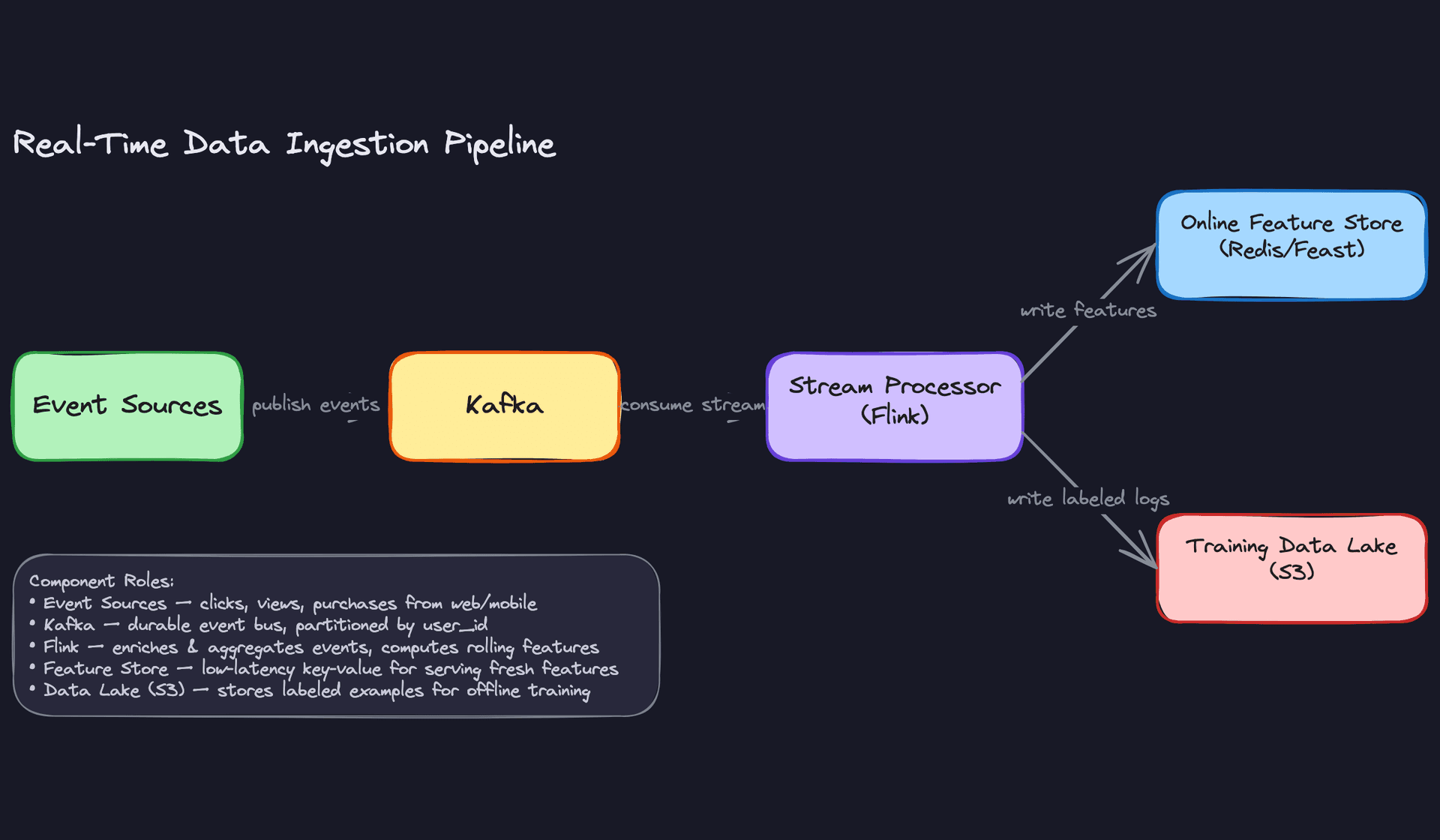
The pipeline ties all of this together. Raw events hit Kafka, get enriched and deduplicated by Flink, then split into two paths: one writes fresh features to Redis for online serving, and the other writes cleaned, labeled, versioned training examples to the data lake. Your training jobs read from the lake, never from the live feature store, which keeps your offline and online environments cleanly separated.
Feature Engineering
Good features beat better models almost every time. Before you touch model architecture, you need to know exactly what signals you're feeding in, where they come from, and how you guarantee consistency between training and serving.
Feature Categories
User Features
These capture who the user is and what they've done historically.
| Feature | Type | How It's Computed |
|---|---|---|
user_embedding | float[128] | Two-tower model trained weekly; stored in Redis online store, indexed in FAISS for ANN search |
30d_click_count | int | Spark batch job over interaction logs, daily refresh |
preferred_categories | float[50] | Weighted category counts over last 90 days, normalized |
account_age_days | int | Derived from signup timestamp at request time |
avg_session_length_7d | float | Flink rolling aggregate over session events |
The embedding is the most valuable signal here. A 128-dimensional vector captures latent taste in a way that no hand-crafted feature can. But it's also the most dangerous for skew, since it's generated offline and must be versioned alongside the model that consumes it.
One clarification worth making explicit: FAISS is an approximate nearest neighbor index used during candidate generation to find items similar to a user's embedding. For the ranking stage, you retrieve the embedding directly by user_id from Redis. These are two different access patterns served by two different systems.
Item Features
These describe what you're ranking, independent of any specific user.
| Feature | Type | How It's Computed |
|---|---|---|
item_embedding | float[128] | Same two-tower training run as user embeddings; stored in Redis, indexed in FAISS for ANN retrieval |
7d_ctr | float | Click / impression ratio over last 7 days, batch job |
publish_age_hours | float | Computed at request time from item metadata |
content_category | int[] | Multi-hot encoding from item catalog, static |
inventory_score | float | Business rule: penalizes out-of-stock or low-supply items |
Freshness matters here in two senses. First, the feature values themselves need to be recent (a 7-day CTR computed last week is stale). Second, new items have no CTR history at all, which is your cold-start problem for items. More on that in the expectations section.
Contextual Features
Context is what makes the same user get different recommendations at 7am on mobile versus 9pm on a desktop.
hour_of_day(int, 0-23): computed at request timeday_of_week(int): computed at request timedevice_type(categorical: mobile/tablet/desktop): from request headerssession_item_views(int[]): items viewed in the current session, maintained in a short-lived session store (Redis with 30-minute TTL)geo_region(categorical): from IP lookup, cached per user
These are cheap to compute and high-signal. Don't skip them.
Cross Features and Interactions
Cross features capture the relationship between a specific user and a specific item. They're the most expensive to compute but often the most predictive.
user_item_affinity_score(float): dot product of user and item embeddings, computed at serving timecategory_match_score(float): overlap between user's preferred categories and item's categorieshistorical_interaction_type(categorical: clicked/purchased/skipped/none): looked up from an interaction history storeco-engagement_score(float): how often users similar to this user engaged with this item, updated daily via batch job
The affinity score is just a dot product, so it's fast. The co-engagement score requires a precomputed user-neighborhood lookup, which means another Redis key per user. Budget for that storage cost.
Feature Computation
The right computation tier depends on two things: how fast the signal changes, and how much latency you can afford to spend retrieving it.
Batch Features
Batch features are your foundation. A Spark job runs on a schedule (typically nightly) over the full interaction log in S3, computes aggregates like 30d_click_count or preferred_categories, and writes results to the offline feature store as Parquet partitioned by user_id and date. A separate write pushes the latest values to the online store (Redis) so they're available at serving time.
The key discipline here is idempotency. Your Spark job should produce the same output if re-run on the same input. This matters when you need to backfill features for retraining.
# Spark batch feature computation example
from pyspark.sql import functions as F

user_features = (
    interactions_df
    .filter(F.col("event_date") >= F.date_sub(F.current_date(), 30))
    .groupBy("user_id")
    .agg(
        F.count("*").alias("30d_click_count"),
        F.countDistinct("item_id").alias("30d_unique_items"),
        F.collect_set("category_id").alias("engaged_categories")
    )
    .withColumn("feature_timestamp", F.current_timestamp())
)

# Write to offline store (Parquet on S3)
user_features.write.partitionBy("date").parquet("s3://features/user/batch/")

# Write latest to online store via Feast push API
feast_store.write_to_online_store("user_batch_features", user_features.toPandas())
Near-Real-Time Features
Some signals go stale in minutes. A user who just clicked three items in the "running shoes" category is telling you something right now. A daily batch job won't capture that.
Kafka feeds raw interaction events into a Flink job that maintains rolling windows. Every time a new event arrives, Flink recomputes the window aggregate and pushes the result to Redis. The latency from user action to updated feature is typically 5-15 seconds.
# Flink streaming feature: items viewed in last 10 minutes
# Pseudocode for the windowed aggregation

env = StreamExecutionEnvironment.get_execution_environment()

click_stream = (
    env
    .add_source(KafkaSource("user_interactions"))
    .key_by("user_id")
    .window(SlidingEventTimeWindows.of(Time.minutes(10), Time.minutes(1)))
    .aggregate(RecentItemsAggregator())  # collects item_ids in window
)

click_stream.add_sink(RedisSink(key_pattern="user:{user_id}:recent_items"))
Key insight: The most common failure mode in ML systems is training-serving skew. Features computed differently in batch training versus online serving will silently corrupt your model. Always design for consistency: the same feature definition, the same aggregation window, the same null-handling logic in both paths.
Real-Time Features
A small set of features can only be computed at request time because they depend on information that doesn't exist until the request arrives.
publish_age_hours is the cleanest example: you compute it as (now - item.published_at) / 3600. No precomputation needed. Similarly, user_item_affinity_score is just a dot product between two embeddings you've already fetched, so you compute it inline in the personalization service rather than storing a value per (user, item) pair (that would be billions of keys).
Keep this category small. Every computation you add here is on the critical path for your p99 latency.
Feature Store Architecture
You need two stores, not one. The offline store serves training; the online store serves inference. They have completely different access patterns.
The online store (Redis or DynamoDB) is a key-value lookup: give it a user_id, get back a feature vector in under 5ms. Redis works well here because you can pack a user's entire feature vector into a single hash key and retrieve it in one round trip. At 100M users with ~1KB of features each, you're looking at roughly 100GB of Redis memory, which is manageable with a few large instances. User and item embeddings live here too, retrieved directly by ID during ranking.
The offline store (Parquet files on S3, or a columnar warehouse like BigQuery) stores the full historical record of feature values, partitioned by date. This is what you join against your training logs when you're building a training dataset. It needs to support time-travel queries: "what were this user's features at 2:47pm on March 3rd?" Without that, you'll accidentally leak future information into your training data.
Feast handles both stores under a unified API and enforces point-in-time correctness during training data retrieval. Here's what that looks like:
from feast import FeatureStore
from datetime import datetime
import pandas as pd

store = FeatureStore(repo_path=".")

# Training: point-in-time correct feature retrieval
# entity_df contains user_id + the exact timestamp of each training example
entity_df = pd.DataFrame({
    "user_id": ["u1", "u2", "u3"],
    "event_timestamp": [
        datetime(2024, 3, 3, 14, 47),
        datetime(2024, 3, 3, 15, 12),
        datetime(2024, 3, 4, 9, 5),
    ]
})

training_features = store.get_historical_features(
    entity_rows=entity_df,
    features=[
        "user_batch_features:30d_click_count",
        "user_stream_features:recent_item_views",
        "user_batch_features:preferred_categories",
    ]
).to_df()
# Feast looks up the feature value that was valid AT event_timestamp,
# not the current value. This is what prevents label leakage.

# Serving: fetch current features for a live request
online_features = store.get_online_features(
    features=["user_batch_features:30d_click_count"],
    entity_rows=[{"user_id": "u1"}]
).to_dict()
The discipline that prevents skew is simple but easy to skip: every feature definition lives in the feature store registry, and both the training pipeline and the serving code read from that same registry. If you compute a feature ad-hoc in a Jupyter notebook for training and then reimplement it in the serving layer, you will get skew. It's not a question of if.
┌─────────────────────────────────────────────────────────────────────────────┐
│                         FEATURE PIPELINE OVERVIEW                           │
│                                                                             │
│  Data Sources          Processing Tier        Feature Stores                │
│  ─────────────         ───────────────        ──────────────                │
│                                                                             │
│  S3 Interaction  ───►  Spark (nightly)  ────► Offline Store (S3/Parquet)   │
│  Logs                  batch aggregates        partitioned by date          │
│                              │                        │                     │
│                              │                        │ point-in-time       │
│                              ▼                        │ correct joins       │
│  Kafka Event     ───►  Flink (streaming) ──┐          ▼                    │
│  Stream                rolling windows     │   ┌─────────────────┐         │
│                                            └──►│  Online Store   │         │
│  Request         ───►  Inline computation  ──► │  (Redis)        │         │
│  Context               at serving time         └────────┬────────┘         │
│                                                         │                  │
│                                                         │ <5ms lookup      │
│                                                         ▼                  │
│                                               ┌──────────────────┐         │
│                                               │  Consumers       │         │
│                                               │                  │         │
│                                               │  Training        │◄── S3   │
│                                               │  Pipeline        │         │
│                                               │                  │         │
│                                               │  Ranking         │◄── Redis│
│                                               │  Service         │         │
│                                               │                  │         │
│                                               │  Candidate       │◄── FAISS│
│                                               │  Generation      │  (ANN)  │
│                                               └──────────────────┘         │
└─────────────────────────────────────────────────────────────────────────────┘
The diagram makes one thing obvious that's easy to miss in prose: FAISS sits alongside the online store, not inside it. Candidate generation queries FAISS to find the top-K nearest neighbors for a user embedding. Ranking then fetches full feature vectors for those candidates from Redis by ID. Two different systems, two different access patterns, both needed.
Freshness Tradeoffs in Practice
When an interviewer asks "how fresh do your features need to be?", don't give a generic answer. Reason through the signal value versus the cost.
A user's 30-day purchase history changes slowly. Running that as a daily batch job is fine, and the cost of a near-real-time version (Flink job, Redis writes, extra infrastructure) isn't worth it. On the other hand, "items viewed in the last 10 minutes" is highly predictive of immediate intent and goes stale fast. That one belongs in the streaming tier.
The practical framework: if a feature's value can change meaningfully within your retraining cadence (say, daily), you need streaming. If it changes on a weekly or monthly timescale, batch is fine. If it only exists at request time, compute it inline.
Common mistake: Candidates design a feature pipeline where everything goes through Flink in real time. That's expensive and operationally complex. Most features don't need sub-minute freshness. Batch the slow-moving ones, stream the fast-moving ones, and compute the trivial ones at request time.
Model Selection & Training
Start simple. Every production personalization system at a company like Netflix or Uber began with something embarrassingly basic, and that's not a mistake. It's a strategy.
The Baseline: Logistic Regression
Before you touch a neural network, your baseline should be logistic regression over hand-crafted features: user's historical CTR, item popularity, time-of-day buckets, and a few user-item interaction counts. It trains in minutes, is trivially debuggable, and gives you a performance floor to beat.
In an interview, proposing a baseline first signals maturity. It shows you understand that a model you can't explain or debug is a liability in production, not an asset.
Tip: When the interviewer asks "what model would you use?", don't jump straight to transformers. Say "I'd start with logistic regression to establish a baseline, then move to GBDT, then consider a deep model if the complexity is justified." That progression earns more points than naming the fanciest architecture.
Two-Stage Architecture: Retrieval Then Ranking
With millions of items in the catalog, you can't score every item for every user on every request. The solution is a two-stage pipeline.
Stage 1: Candidate Generation. Retrieve a small set of plausible candidates (typically 100 to 1000 items) from the full catalog using a fast, approximate method. Speed matters more than precision here. You're casting a wide net.
Stage 2: Ranking. Score only those candidates with a more expressive model that can capture complex feature interactions. This is where you spend your latency budget on quality.
Some systems add a third stage: re-ranking, which applies business rules, diversity constraints, or policy filters after the ML model scores. Think "don't show the same brand three times in a row" or "boost sponsored items by a fixed factor." Keep this logic outside the model so it's auditable and adjustable without retraining.
Stage 1: Two-Tower Model for Candidate Generation
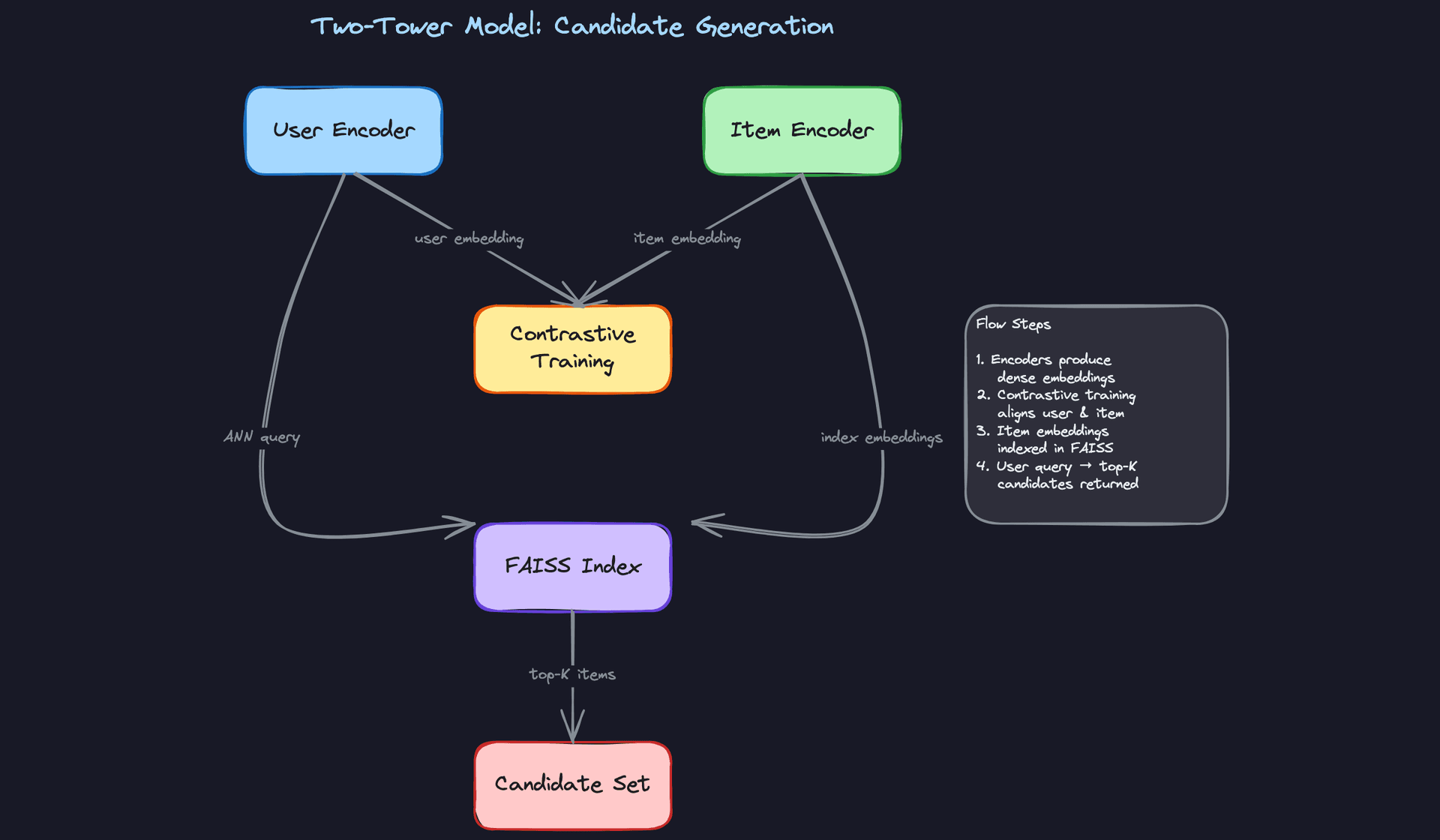
The two-tower model is the standard architecture for candidate generation at scale. You train two separate neural encoders: one for users, one for items. Both map their respective inputs into the same embedding space, and you optimize for high dot-product similarity between a user and items they interacted with.
User tower inputs: - User ID embedding (learned, dim=64) - Recent interaction history (average pooled item embeddings, dim=64) - Demographics and device type (one-hot, dim=20) - Session-level signals: time since last visit, session length (dim=5)
Item tower inputs: - Item ID embedding (learned, dim=64) - Content features: category, tags, text embedding from a pretrained encoder (dim=128) - Popularity and freshness signals (dim=10)
Both towers output a 128-dimensional L2-normalized embedding vector.
Loss function: In-batch softmax with negative sampling. For each positive (user, item) pair in a batch, all other items in the batch serve as negatives. This is computationally efficient and works well when your batch size is large enough to provide hard negatives.
import torch
import torch.nn.functional as F

def two_tower_loss(user_embeddings, item_embeddings, temperature=0.07):
    # user_embeddings: [batch_size, embed_dim]
    # item_embeddings: [batch_size, embed_dim]

    # Normalize
    user_embeddings = F.normalize(user_embeddings, dim=-1)
    item_embeddings = F.normalize(item_embeddings, dim=-1)

    # Similarity matrix: [batch_size, batch_size]
    logits = torch.matmul(user_embeddings, item_embeddings.T) / temperature

    # Diagonal entries are the positive pairs
    labels = torch.arange(logits.size(0), device=logits.device)

    loss = F.cross_entropy(logits, labels)
    return loss
At inference time, you compute user embeddings on the fly and query a FAISS index containing all pre-computed item embeddings. ANN retrieval over 10 million items takes under 10ms on a single CPU with HNSW indexing.
Common mistake: Candidates describe the two-tower architecture but forget to mention that item embeddings are indexed offline and refreshed on a schedule. The FAISS index doesn't update in real time. If you add new items, there's a lag before they appear in retrieval results. Interviewers will ask about this. Say you handle it with a "fresh items" side channel that injects new catalog entries directly into the candidate set, bypassing ANN retrieval.
Stage 2: Ranking Model
The ranking stage receives the candidate set from retrieval and produces a relevance score for each item. This is where you can afford more compute per item.
The production workhorse: LightGBM. For most teams, a gradient boosted decision tree model is the right call. It handles mixed feature types natively, trains fast, serves fast (in-process, no network hop), and is interpretable enough that you can debug mispredictions. LightGBM in particular handles sparse categorical features efficiently and regularizes well on large feature sets.
When to go deeper: DCN v2. If you have strong evidence that feature interactions matter and you have the infrastructure to support it, a Deep and Cross Network (DCN v2) captures explicit high-order feature crosses without requiring manual feature engineering. The cross network learns interactions like "user who bought electronics AND is browsing on mobile AND it's a weekend" automatically.
Ranking model inputs (assembled per candidate item): - User features from the feature store (dim ~150) - Item features from the feature store (dim ~100) - User-item cross features: user's historical CTR on this item's category, item's CTR for this user's demographic segment (dim ~30) - Context features: time of day, device, position in the request (dim ~10)
Output: A single scalar score representing predicted CTR or predicted conversion probability, depending on your business objective. For a feed ranking system, you typically optimize for a weighted combination: score = w1 * pCTR + w2 * pDwell + w3 * pShare.
Loss function: Binary cross-entropy for pointwise ranking (treating each item as an independent click/no-click prediction). If you want to directly optimize ranking quality, pairwise losses like BPR (Bayesian Personalized Ranking) or listwise losses like ListNet work better but are harder to train stably at scale. Most production systems start pointwise and move to pairwise once the infrastructure is solid.
# LightGBM ranking model config
import lightgbm as lgb

params = {
    "objective": "binary",          # pointwise CTR prediction
    "metric": ["auc", "binary_logloss"],
    "num_leaves": 127,
    "learning_rate": 0.05,
    "feature_fraction": 0.8,
    "bagging_fraction": 0.8,
    "bagging_freq": 5,
    "min_child_samples": 100,       # prevents overfitting on rare users
    "lambda_l1": 0.1,
    "lambda_l2": 0.1,
    "num_threads": 16,
}

model = lgb.train(
    params,
    train_data,
    num_boost_round=500,
    valid_sets=[val_data],
    callbacks=[lgb.early_stopping(50), lgb.log_evaluation(50)],
)
Training Pipeline
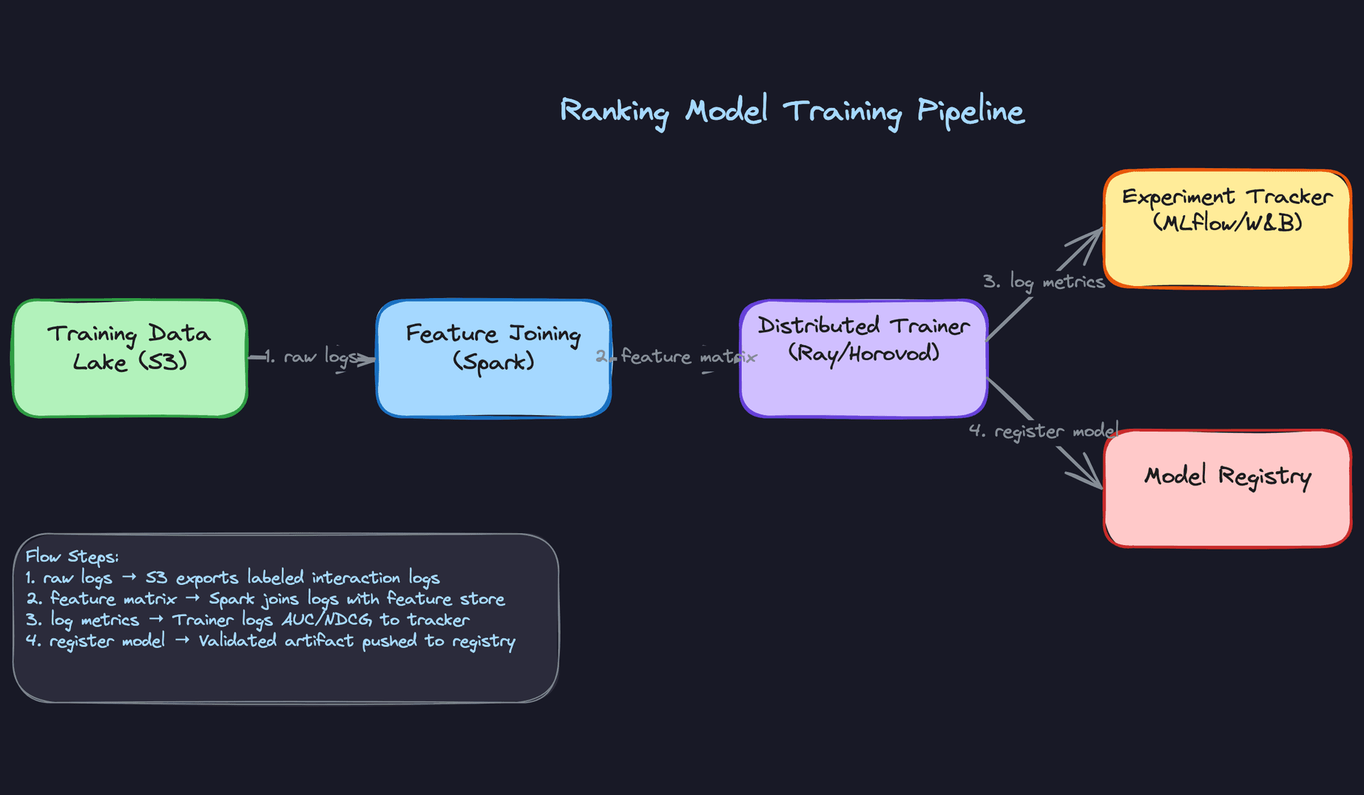
Infrastructure. LightGBM trains on a single large machine (64-core, 512GB RAM) for most catalog sizes. If you move to a deep ranking model, you need distributed training. Ray Train or Horovod handles data-parallel training across multiple GPU workers, with PyTorch's DistributedDataParallel managing gradient synchronization.
For the two-tower model, a 4xA100 setup is sufficient for most production scales. Expect training runs of 2 to 6 hours on 500M interaction examples.
Training schedule. Retrain the ranking model daily. User preferences shift, item catalogs change, and a week-old model will start to show measurable CTR degradation. The two-tower model is more expensive to retrain, so weekly full retrains with daily incremental embedding updates is a reasonable cadence.
Full retraining rebuilds the model from scratch on a rolling window of data. Incremental retraining (fine-tuning from the previous checkpoint) is faster but risks compounding errors if the data distribution has shifted significantly.
Key insight: The choice between full retraining and incremental fine-tuning isn't just about compute cost. It's about how much distribution shift you've accumulated. If your data pipeline had a bug for 48 hours, you want a full retrain, not a fine-tune on corrupted data.
Data windowing. Don't train on all historical data. Use a rolling window of the last 30 to 90 days for the ranking model. Data older than that reflects user preferences and item catalogs that no longer exist. The right window length is empirical: compare offline AUC and online CTR for models trained on 30-day vs. 60-day vs. 90-day windows.
One exception: cold-start handling. You want to keep some older data to ensure rare user segments and long-tail items have enough training examples. A practical approach is to use a 30-day primary window with a 10% sample from the past year as a regularization supplement.
Hyperparameter tuning. Use Bayesian optimization (Optuna or Ray Tune) over a fixed validation set. The key parameters to tune for LightGBM are num_leaves, learning_rate, min_child_samples, and the regularization terms. For deep models, focus on learning rate schedule, embedding dimensions, and dropout rates. Don't tune on the test set. Ever.
Offline Evaluation
AUC is not enough. A model with 0.78 AUC that systematically misfires on mobile users or new items is a production incident waiting to happen.
Primary metrics: - AUC-ROC: overall discrimination ability. Useful for comparing model versions but doesn't tell you about calibration. - Log loss: measures calibration quality. If your model predicts 0.8 CTR but actual CTR is 0.3, your downstream score blending will be wrong. - NDCG@K: measures ranking quality directly. More aligned with the actual user experience than pointwise AUC. - MRR (Mean Reciprocal Rank): useful when the user cares primarily about the first relevant result.
Evaluation methodology. Use time-based splits, not random splits. If you randomly shuffle your data and split 80/20, you'll leak future information into training (a user's future clicks informing their past feature values). Always train on data from time T-N to T, and evaluate on data from T to T+M.
Backtesting is your friend here. Simulate what your model would have ranked on a held-out day of traffic, compare against what actually got clicked, and compute NDCG. It's not a perfect proxy for online performance, but it catches regressions before they reach users.
Baseline comparisons. Every model evaluation should include: 1. Popularity-based ranker (most clicked items globally) 2. Logistic regression baseline 3. Previous production model
If your new model doesn't beat the previous production model by at least 0.5% NDCG, don't ship it. The noise floor in offline evaluation is real.
Error analysis. Slice your evaluation results. Don't just look at aggregate AUC. Break it down by: - New users vs. established users (cold-start performance is almost always worse) - Item age (fresh items have sparse interaction data; your model will underrank them) - Device type (mobile vs. desktop user behavior differs significantly) - Interaction type (clicks vs. purchases; the model may be well-calibrated for clicks but not conversions)
The failure modes you'll typically find: the model over-ranks popular items (popularity bias from training data), under-ranks new items (sparse signal), and performs poorly on users with unusual taste profiles (distribution tail). Document these before the interview. Interviewers who ask "what are the failure modes of your model?" are separating senior candidates from the rest.
Tip: Interviewers want to see that you evaluate models rigorously before deploying. "It has good AUC" is not enough. Discuss calibration (is predicted CTR 0.3 actually 30% click rate?), fairness slices (does the model perform equally across user demographics?), and failure modes (what does it get wrong and why?). A candidate who proactively raises these points without being asked is a strong signal for senior and above.
Exploration vs. Exploitation
One thing the offline metrics won't tell you: whether your model is creating a filter bubble. A perfectly optimized ranker will keep showing users the same types of content they've always clicked on, which maximizes short-term CTR but degrades long-term engagement.
The standard fix is to inject exploration at serving time. Epsilon-greedy is the simplest approach: with probability epsilon (say 5%), replace a ranked item with a randomly sampled one from the candidate set. This gathers signal on items the model hasn't seen the user interact with.
For more principled exploration, a contextual bandit layer sits on top of the ranking model and uses Thompson Sampling or UCB to balance exploitation of high-confidence predictions with exploration of uncertain ones. This is what systems like Google's recommendation engine and Spotify's Discover Weekly use under the hood.
The key point for the interview: exploration is not a nice-to-have. Without it, your training data becomes a self-reinforcing loop. The model learns what it already showed users, not what users would have liked if shown something different.
Inference & Serving
Getting a model to 95% AUC in a notebook is the easy part. Getting it to respond in under 100ms for 50,000 users simultaneously, without dropping requests when a downstream service hiccups, is where the real engineering lives.
Serving Architecture
For a real-time personalization engine, online inference is non-negotiable. You're personalizing per-user, per-request, with context signals (current session, device, time of day) that only exist at request time. Batch inference would mean pre-computing rankings for every user against every item on a schedule, which doesn't scale to a catalog of millions and goes stale within minutes.
The serving path has four stages, and they need to run in parallel wherever possible.
Request
   │
   ▼
┌─────────────────────┐
│     API Gateway     │  auth, rate-limit, route
└─────────┬───────────┘
          │
          ▼
┌─────────────────────┐
│ Personalization Svc │  owns the latency budget
└──────┬──────────────┘
       │  fires in parallel
       ├──────────────────────────────┐
       ▼                              ▼
┌─────────────┐              ┌────────────────┐
│  Redis      │              │  FAISS Index   │
│ (features)  │              │ (ANN retrieval)│
└──────┬──────┘              └───────┬────────┘
       └──────────┬───────────────────┘
                  │  assemble feature matrix
                  ▼
        ┌──────────────────┐
        │  Ranking Model   │  Triton / TFServing / in-process
        │     Server       │
        └────────┬─────────┘
                 │
                 ▼
        ┌──────────────────┐
        │  Post-processing │  dedup, diversity, sponsored items
        └────────┬─────────┘
                 │
                 ▼
            Response
The API gateway receives a request with user_id, context, and optionally a surface identifier (home feed vs. search). It authenticates, rate-limits, and hands off to the personalization service, which owns the latency budget from that point forward.
Personalization Service API
The service exposes a single ranking endpoint. Keep the contract simple.
POST /v1/personalize
{
  "user_id": "u_8f3a92c1",
  "surface": "home_feed",
  "context": {
    "session_id": "s_4d71b",
    "device_type": "mobile",
    "timestamp_ms": 1718200000000,
    "geo_region": "us-west-2"
  },
  "request_config": {
    "num_results": 20,
    "candidate_pool_size": 200,
    "max_latency_ms": 100
  }
}
HTTP 200
{
  "user_id": "u_8f3a92c1",
  "ranked_items": [
    { "item_id": "i_001", "score": 0.94, "rank": 1 },
    { "item_id": "i_047", "score": 0.91, "rank": 2 }
  ],
  "model_version": "ranker-v42",
  "served_by": "champion",
  "latency_breakdown_ms": {
    "feature_fetch": 8,
    "candidate_retrieval": 4,
    "ranking_inference": 18,
    "post_processing": 3
  }
}
Returning model_version and served_by in every response is not optional. You need this for debugging, for correlating online metrics back to a specific model, and for confirming that your canary traffic is actually hitting the right model.
The personalization service fires two requests in parallel: a feature fetch from Redis (user features, pre-computed item features) and a candidate retrieval from the FAISS index (top-K items via ANN lookup on the user embedding). Both should complete in under 15ms combined. Once candidates are back, the service assembles the feature matrix and calls the ranking model server.
Here's what that parallel fetch looks like in practice:
import asyncio
from typing import Optional

async def build_ranking_request(
    user_id: str,
    context: dict,
    candidate_pool_size: int = 200,
) -> dict:
    # Fire feature fetch and ANN retrieval in parallel
    user_features_task = asyncio.create_task(
        feature_store.get_user_features(user_id)
    )
    candidates_task = asyncio.create_task(
        ann_index.retrieve(
            user_id=user_id,
            top_k=candidate_pool_size,
        )
    )

    # Both must complete within 15ms or we fall back
    try:
        user_features, candidates = await asyncio.wait_for(
            asyncio.gather(user_features_task, candidates_task),
            timeout=0.015,
        )
    except asyncio.TimeoutError:
        return await fallback_popularity_ranker(context)

    # Batch-fetch item features for all candidates in one Redis pipeline
    item_features = await feature_store.get_item_features_batch(
        item_ids=[c.item_id for c in candidates]
    )

    return assemble_feature_matrix(user_features, item_features, candidates, context)
The timeout on the gather call is the key detail. You don't wait indefinitely for a slow feature store; you fall back. More on fallback behavior below.
For the ranking model, your choice of serving infrastructure matters a lot:
- Triton Inference Server is the right default for neural ranking models. It handles dynamic batching, supports TensorRT optimization, and runs on GPU. If your ranker is a deep model (Wide & Deep, DCN, transformer-based), Triton is where you want to be.
- TFServing works well if your team is already TensorFlow-native. It's more opinionated but has solid versioning and model warm-up support.
- LightGBM in-process is the right call for GBDT rankers. Calling a separate model server for a tree model adds 5-10ms of network overhead for no reason. Load the model artifact directly into the personalization service process and call it as a library.
Don't over-engineer the serving stack for your model type. A LightGBM model doesn't need a GPU server.
Latency Budget
You have 100ms p99 to work with. Here's how to spend it:
| Stage | Budget | Notes |
|---|---|---|
| Feature fetch (Redis) | ~10ms | Batch key lookup; pipeline the Redis calls |
| ANN candidate retrieval (FAISS) | ~5ms | Pre-built index; HNSW is faster than flat |
| Ranking model inference | ~20ms | Batched; GPU if neural, in-process if GBDT |
| Post-processing + business rules | ~5ms | Dedup, diversity filters, sponsored item injection |
| Network + serialization overhead | ~10ms | Minimize hops; keep services co-located |
| Buffer | ~50ms | For tail latency, GC pauses, cold starts |
The buffer is not slack. P99 latency is driven by the worst 1% of requests, which hit cold caches, large candidate sets, and JVM GC pauses all at once. If your median is 40ms, your p99 will still blow past 100ms without that buffer.
Optimization
Model Optimization
The fastest inference is inference you don't do. A response cache with a short TTL (30-60 seconds) on the ranked output handles repeat requests from the same user in the same session. This is especially effective on high-traffic surfaces like a home feed that refreshes frequently.
For the model itself, the optimization hierarchy looks like this. Start with quantization: converting FP32 weights to INT8 cuts memory bandwidth by 4x and typically costs less than 1% AUC on ranking models. TensorRT handles this automatically during Triton model compilation. If you need to go further, knowledge distillation trains a smaller student model to mimic a larger teacher; this is worth the effort if your neural ranker is the bottleneck. Pruning is usually the last resort since it requires more careful fine-tuning to recover accuracy.
For GBDT models, the main lever is limiting tree depth and number of estimators. A LightGBM model with 500 trees and max depth 6 will score 1,000 candidates in under 5ms on a single CPU core.
Batching
Dynamic batching is critical for GPU utilization. Instead of scoring one request at a time, Triton accumulates requests over a short window (1-5ms) and scores them together. A batch of 32 requests takes roughly the same GPU time as a batch of 1 on modern hardware. The tradeoff is added latency from the wait window, so tune the max batch wait time against your p99 target.
# triton model config for the ranking model
name: "deep_ranker"
backend: "tensorrt"
max_batch_size: 64

dynamic_batching {
  preferred_batch_size: [16, 32, 64]
  max_queue_delay_microseconds: 2000   # 2ms max wait to fill a batch
}

instance_group [
  { kind: KIND_GPU, count: 2 }         # two model instances per GPU
]
On the CPU side, batching helps less. If you're serving LightGBM in-process, just score each request independently and scale horizontally.
GPU vs. CPU
Neural ranking models with large embedding tables almost always benefit from GPU serving. The memory bandwidth for embedding lookups is the bottleneck, and GPU HBM is 10-20x faster than CPU DRAM for this pattern.
For shallow models (logistic regression, GBDT, small MLPs), CPU serving is cheaper and often faster end-to-end once you account for the overhead of moving data to GPU memory. Don't default to GPU just because it sounds more serious.
Fallback Strategies
Your personalization service needs to degrade gracefully, not fail loudly.
async def get_rankings(
    user_id: str,
    context: dict,
    num_results: int = 20,
) -> RankingResponse:
    # Attempt full personalized ranking
    try:
        feature_matrix = await build_ranking_request(user_id, context)
        scores = await ranking_model.score(feature_matrix)
        return RankingResponse(
            items=scores.top_k(num_results),
            served_by="champion",
        )

    except FeatureStoreUnavailable:
        # Try stale local cache before giving up on personalization
        stale = local_cache.get(user_id, max_age_seconds=3600)
        if stale:
            scores = await ranking_model.score(stale)
            return RankingResponse(
                items=scores.top_k(num_results),
                served_by="champion_stale_features",
            )
        # Feature store down and no cache; fall through

    except (ModelServerTimeout, ModelServerUnavailable):
        pass  # fall through to popularity ranker

    # Final fallback: pre-computed global top-K
    popular_items = popularity_cache.get_top_k(
        surface=context["surface"],
        k=num_results,
    )
    return RankingResponse(items=popular_items, served_by="popularity_fallback")
If the ranking model server is unavailable or exceeds its timeout, fall back to a popularity-based ranker. Pre-compute a global top-K list (updated every few minutes) and serve that. Users get a reasonable experience; you don't get a P0 incident.
If the feature store is unavailable, serve with stale features from a local in-memory cache rather than returning an error. A 5-minute-old user feature vector is far better than a 500 response. Set a max staleness threshold (say, 1 hour) beyond which you fall back to the popularity ranker.
Common mistake: Candidates design the happy path in detail and then say "we'd add retries and timeouts" as an afterthought. Interviewers at senior levels expect you to specify the fallback behavior concretely: what triggers it, what the user sees, and how you recover.
Online Evaluation & A/B Testing
Offline metrics (AUC, NDCG) tell you the model learned something. Online metrics tell you whether it actually helps users. The two can diverge badly, and they often do.
Traffic Splitting and Experiment Assignment
Assign users to experiment buckets using a deterministic hash of user_id + experiment_id. This ensures the same user always sees the same model version within an experiment, which prevents the "flickering" problem where a user sees different rankings on consecutive page loads.
Keep experiment buckets mutually exclusive at the user level. If you're running three experiments simultaneously, a user should be in at most one. Overlapping experiments contaminate your metric estimates.
The minimum detectable effect drives your sample size calculation. For a 1% relative lift in CTR on a surface with 2% baseline CTR, you typically need several hundred thousand users per variant to reach 95% confidence within a week. Know this number before you start the experiment, not after.
Online Metrics
Track metrics at two levels. Business metrics (CTR, conversion rate, session length, revenue per session) are the ultimate arbiter but are noisy and slow to move. Model health metrics (prediction score distribution, ranking position of clicked items, feature null rates) are faster to detect problems and easier to debug.
Watch for novelty effects: a new model often shows a short-term CTR bump just because it's different. Run experiments for at least one full week to wash out day-of-week effects and novelty bias before making a promotion decision.
Ramp-Up and Rollback
Start at 1% traffic. Let it run for 24 hours and check that model health metrics look sane (no score distribution collapse, no latency regression). If clean, move to 10%, then 50%, then 100%, with a hold at each stage.
Define rollback triggers before you start the ramp. Automated rollback should fire if p99 latency increases by more than 20ms, if CTR drops more than 5% relative to control, or if error rate exceeds a threshold. These numbers should be agreed on with the team before deployment, not negotiated during an incident.
Interleaving for Ranking Systems
Standard A/B testing for ranking has a sensitivity problem: the effect of a ranking change on a single user session is small and noisy, so you need huge sample sizes. Interleaving solves this.
In an interleaved experiment, you merge the ranked lists from two models for the same user in the same request, alternating items from each model's ranking (with team assignment tracked per item). You then measure which model's items got more clicks. Because both models compete for the same user's attention in the same session, the signal-to-noise ratio is dramatically better, often 100x more sensitive than standard A/B testing. Netflix and LinkedIn have published extensively on this pattern for recommendation systems.
The catch: interleaving only tells you which model is relatively better, not the absolute effect size. Use it for fast model selection, then confirm the magnitude of the effect with a standard A/B test before full rollout.
Deployment Pipeline
New Model Artifact
       │
       ▼
┌─────────────────────────┐
│   Validation Gates      │  offline regression, latency benchmark,
│                         │  feature coverage check
└──────────┬──────────────┘
           │ pass
           ▼
┌─────────────────────────┐
│   Shadow Scoring        │  mirror live traffic; log only, no user impact
│   (24+ hours)           │
└──────────┬──────────────┘
           │ score distributions look healthy
           ▼
┌─────────────────────────┐
│   Canary: 1%            │  24h hold; automated rollback active
└──────────┬──────────────┘
           │ metrics clean
           ▼
┌─────────────────────────┐
│   Ramp: 10% → 50%       │  24h hold at each stage; human review gate
└──────────┬──────────────┘
           │ approved
           ▼
┌─────────────────────────┐
│   Full Traffic: 100%    │  previous version stays warm for 48h
└─────────────────────────┘
           │ rollback trigger fires at any stage
           ▼
┌─────────────────────────┐
│   Rollback              │  config change; < 5 min; previous version warm
└─────────────────────────┘
Validation Gates
A model should never reach production without passing a pre-deployment checklist. At minimum:
- Offline regression check: new model AUC must be within 0.5% of the current production model on a held-out evaluation set. A drop here means something went wrong in training.
- Latency benchmark: score a fixed batch of 1,000 requests on the target serving hardware. P99 must be within budget.
- Shadow scoring comparison: run the new model in shadow mode (see below) for at least 24 hours and compare prediction score distributions against the champion model. A bimodal shift or score collapse is a red flag.
- Feature coverage check: confirm that all features the new model expects are available in the online feature store with acceptable null rates.
Fail any of these and the deployment stops. Automate all of them.
def run_validation_gates(
    new_model: ModelArtifact,
    champion_model: ModelArtifact,
    eval_dataset: EvalDataset,
    serving_hardware: HardwareSpec,
) -> ValidationResult:
    results = {}

    # Gate 1: offline regression
    new_auc = evaluate_auc(new_model, eval_dataset)
    champion_auc = evaluate_auc(champion_model, eval_dataset)
    results["auc_regression"] = (champion_auc - new_auc) < 0.005

    # Gate 2: latency benchmark
    p99_ms = benchmark_latency(new_model, serving_hardware, n_requests=1000)
    results["latency_ok"] = p99_ms < LATENCY_BUDGET_MS

    # Gate 3: feature coverage
    missing_features = check_feature_coverage(
        model_feature_schema=new_model.feature_schema,
        online_store=feature_store,
        max_null_rate=0.02,
    )
    results["feature_coverage"] = len(missing_features) == 0

    passed = all(results.values())
    return ValidationResult(passed=passed, details=results)
Shadow Scoring
Before a new model sees any real traffic, mirror a copy of live requests to it. The shadow model scores every request but its output is logged, never shown to users. This lets you validate that the model actually runs in production conditions, with real feature distributions, real request patterns, and real infrastructure load.
Shadow scoring catches a class of bugs that offline evaluation never will: features that exist in training data but are missing or malformed in the online feature store, serialization mismatches between training and serving, and latency regressions that only appear under load.
Run shadow scoring for at least 24 hours before any canary traffic.
Canary Rollout
After shadow scoring passes, route 1% of real traffic to the new model. The canary slice gets real users and real consequences, so your automated rollback triggers must be active from the moment canary traffic starts.
The rollout schedule: 1% for 24 hours, 10% for 24 hours, 50% for 24 hours, 100%. At each stage, a human reviews the metrics dashboard before approving the next step. Fully automated rollout to 100% is a bad idea for ranking models because the business impact of a bad model at full traffic can be severe before automated triggers catch it.
Rollback
Rollback should take under five minutes. That means the previous model version is still deployed and warm, the traffic router can switch back with a config change, and the rollback is triggered either manually or automatically by the metrics controller.
Keep the previous two model versions warm in your serving infrastructure at all times. Cold-starting a model server under incident conditions, while your CTR is tanking, is not a situation you want to be in.
Interview tip: When you describe your deployment pipeline, mention the rollback strategy in the same breath as the rollout strategy. Interviewers notice when candidates only plan for success. Saying "we'd ramp from 1% to 100% with automated rollback if CTR drops more than 5% relative to control" signals production maturity that most candidates skip.
Key insight: The deployment pipeline is where most ML projects fail in practice. A model that can't be safely deployed and rolled back is a model that won't ship.
Monitoring & Iteration
Most personalization systems are designed carefully at launch and then left to quietly degrade. CTR slowly drops, features go stale, and nobody notices until a business review six months later. The teams that avoid this build monitoring and iteration as first-class concerns from day one.
Production Monitoring
There are three distinct failure modes, and they require different detectors.
Data drift is when your input distributions shift. The model itself hasn't changed, but the world has. A new mobile app version changes how session length is computed. A marketing campaign floods the system with a demographic the model has rarely seen. You catch this by tracking feature distributions over time and alerting when a feature's mean, variance, or null rate deviates significantly from a rolling baseline.
Concept drift is subtler. The relationship between features and labels changes. What users clicked on last quarter isn't what they click on now. Your model's AUC on held-out data looks fine, but online CTR is quietly declining. This is why offline metrics alone aren't enough. You need online metric tracking as a primary signal.
Model degradation is the catch-all: online metrics drop without an obvious upstream cause. Sometimes it's concept drift. Sometimes it's a bad feature pipeline. Sometimes a dependency changed and nobody told the ML team. The point is you need enough observability to distinguish between these cases quickly.
Data Monitoring
Track feature null rates, out-of-range values, and schema violations at the feature store boundary. If user_recent_clicks is suddenly null for 15% of requests when it's normally null for 0.5%, something broke upstream. Set hard alerts on null rate thresholds, not just soft warnings.
For distribution drift, Population Stability Index (PSI) is the standard tool. Compute it daily against a reference window (typically the last 30 days of training data). PSI above 0.2 is a meaningful shift; above 0.25 should trigger an investigation.
Tip: Don't alert on every feature independently. You'll drown in noise. Group features by pipeline source and alert at the source level first, then drill down.
Model Monitoring
Log the full prediction score distribution for every model version in production. A ranking model that normally outputs scores between 0.3 and 0.7 suddenly outputting scores clustered near 0.1 is a red flag, even before you see business metric impact.
Track prediction entropy as a proxy for model confidence. A model that's suddenly very uncertain about everything, or conversely very certain about everything, is usually reacting to a distribution shift it wasn't trained to handle.
For performance, you can't always wait for ground-truth labels. Use proxy metrics: click-through rate on top-ranked items, dwell time, and skip rate are available within minutes. Full conversion labels might take days, but these proxies give you an early warning signal.
System Monitoring
The standard infrastructure metrics apply here, but a few deserve special attention for personalization systems specifically.
Feature store hit rate matters a lot. A cache miss on user features means you're either serving stale data or falling back to defaults, both of which silently degrade personalization quality without throwing an error. Track this per feature group, not just overall.
GPU utilization on your Triton or TFServing instances should stay in the 60-80% range under normal load. Consistently above 90% means you're one traffic spike away from latency SLA violations. Consistently below 40% means you're over-provisioned and wasting money.
Track p99 latency end-to-end and per stage. If your total p99 creeps from 80ms to 95ms over two weeks, something is degrading. Knowing whether it's the feature fetch, the ANN lookup, or the model inference tells you exactly where to look.
Alerting Thresholds and Escalation
Set three tiers. Tier 1 (page immediately): p99 latency exceeds SLA, error rate above 1%, feature store unavailable. Tier 2 (alert during business hours): PSI above 0.25 on any critical feature, prediction score distribution shift beyond two standard deviations, CTR drop of more than 5% relative to the control group. Tier 3 (weekly review): gradual metric trends, model age, training data staleness.
The escalation path matters as much as the thresholds. A Tier 1 alert that wakes up an on-call engineer should have a runbook attached. "Model is degrading" is not actionable. "Feature store hit rate dropped to 40%, likely cause is Redis memory eviction, runbook here" is.
Feedback Loops
Every click, purchase, and skip is a training signal. Getting that signal back into the model efficiently is what separates a system that improves from one that stagnates.
User interaction events flow from the client through Kafka and into the same Flink pipeline that powers your online features. The difference is that for training purposes, you're writing labeled examples to the data lake, not just updating feature aggregates. A click on item X for user Y at time T, combined with the feature snapshot that was used to rank X at that moment, becomes a training row.
That last part is critical. You must log the features that were actually served, not recompute them later. Recomputing features after the fact introduces training-serving skew because the feature store has been updated since the request was made. Store the feature snapshot alongside the event.
Feedback Delay Handling
Clicks arrive within seconds. Purchases might arrive within minutes. But some labels take much longer. A subscription conversion might not be attributed for 7 days. A churn signal might take 30 days to confirm.
Don't wait for all labels before training. Use a tiered label strategy: train on immediate feedback (clicks, add-to-cart) for daily model updates, and separately train on delayed feedback (purchases, subscriptions) on a weekly cadence. The daily model captures recency; the weekly model captures quality.
For delayed labels, you need to handle the case where an event arrives after you've already used that example in training with a "no conversion" label. One approach is to use a delayed feedback model that explicitly models the time-to-conversion distribution and corrects for it. The simpler approach is to set a fixed attribution window and accept that you'll miss some late conversions. For most systems, the simpler approach is fine.
Common mistake: Candidates often describe the feedback loop as "events go back to Kafka and retrain the model." That's the skeleton, not the design. The interviewer wants to know how you handle label delay, feature snapshot logging, and negative sampling. Those details are where the real complexity lives.
Closing the Loop
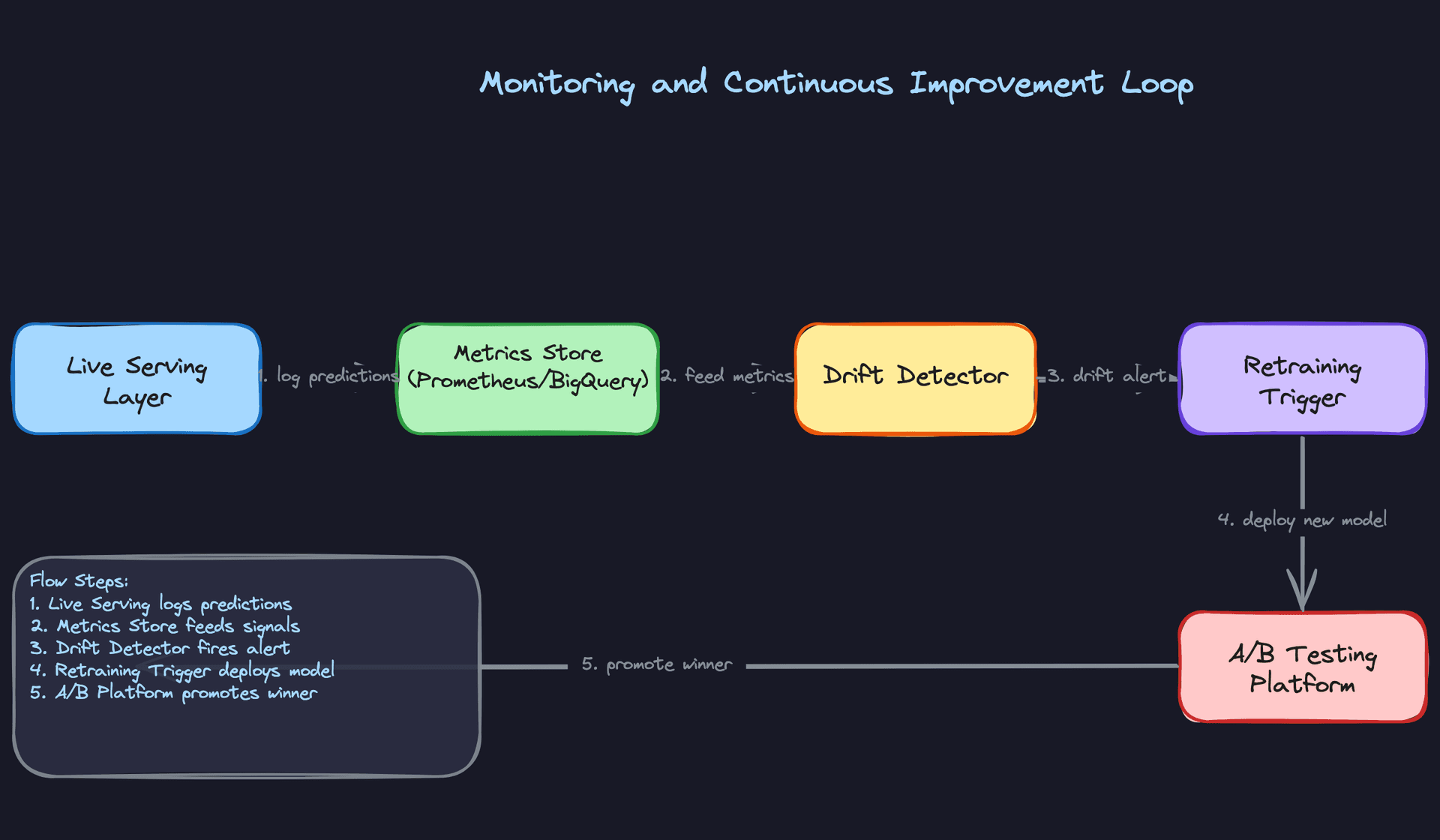
The full cycle looks like this: a drift alert fires because PSI on user_session_length exceeded 0.25. You investigate and confirm that a new app version changed how session length is computed. You fix the feature computation, backfill the affected window in the data lake, trigger an out-of-cycle retraining run, validate the new model in shadow mode, and promote it through canary. The whole loop should take hours, not weeks.
That speed requires automation. Manual retraining pipelines that require an engineer to SSH into a machine and run a script will never close the loop fast enough. Your retraining pipeline should be triggerable by an API call, with the full train-evaluate-register-deploy cycle automated and gated by metric thresholds.
Continuous Improvement
Tip: Staff-level candidates distinguish themselves by discussing how the system improves over time, not just how it works at launch.
Retraining Strategy
Scheduled retraining (daily or weekly) is the baseline. It's predictable, easy to operate, and handles gradual concept drift. Most production systems start here and stay here longer than they should.
Drift-triggered retraining is the upgrade. When your PSI monitor fires or your online metrics drop beyond a threshold, an automated job kicks off a retraining run without waiting for the next scheduled window. This is especially valuable for systems with seasonal patterns or external shocks (a viral news event, a product launch) that invalidate the current model quickly.
The tradeoff is stability. Triggering retraining too aggressively can cause model churn, where the model is constantly changing and you lose the ability to attribute metric changes to specific causes. A reasonable guard is a minimum time between triggered retrains (say, 24 hours) and a requirement that the new model pass shadow evaluation before promotion.
Online learning sits at the far end of the spectrum. Rather than full retraining cycles, you update specific model components (embedding layers, output bias terms) continuously using recent data. This can reduce adaptation latency from hours to minutes. The risk is instability: a bad batch of training data can corrupt the model before you catch it. If you go this route, you need tight guardrails on update magnitude and the ability to instantly roll back to a checkpoint.
Prioritizing Model Improvements
When you have a backlog of potential improvements (new features, architecture changes, data quality fixes), prioritize by expected impact and reversibility.
Data quality fixes first, always. A corrupted feature hurts every model that uses it. Fixing it is high-leverage and low-risk. Architecture changes come last. They're expensive to train, slow to evaluate, and hard to roll back if something goes wrong.
For new features, use offline ablation studies to estimate impact before committing to a full A/B test. If adding user_purchase_history_30d improves offline AUC by 0.5%, it's worth the engineering cost of adding it to the feature pipeline. If the offline lift is negligible, skip it.
Long-Term Evolution
In the first few months, you're mostly fixing data quality issues and closing gaps between offline and online metrics. The model architecture matters less than the pipeline reliability.
By six months, the low-hanging fruit is gone. Improvements come from better feature engineering, more sophisticated architectures (moving from GBDT to a deep ranking model, adding cross features), and tighter exploration-exploitation strategies to reduce filter bubble effects.
At maturity, the biggest gains come from the feedback loop itself. A system that retrains daily with clean labels and good negative sampling will outperform a more sophisticated model trained on stale, biased data. The infrastructure around the model becomes the competitive moat, not the model architecture.
The teams that build the best personalization systems aren't necessarily the ones with the best models. They're the ones who can safely ship a new model every day, measure its impact precisely, and roll back in five minutes when something goes wrong.
What is Expected at Each Level
Interviewers calibrate their expectations based on your level, but the cold-start problem and failure mode reasoning are fair game for everyone. Know those two things cold before you walk in.
Mid-Level
- Sketch the two-stage architecture without being prompted: candidate generation (ANN retrieval or collaborative filtering) feeds a ranking model. If you jump straight to "train a neural net on all items," you've already lost points.
- Name the three feature categories (user, item, context) and give concrete examples of each. "User features like recent click history, item features like category embeddings, context features like time of day" is the right level of specificity.
- Articulate the latency budget. Know that feature retrieval, ANN lookup, model inference, and post-processing each consume a slice of your 100ms SLA, and that you can't spend all of it on the model.
- Explain what a feature store is and why you need one. The answer isn't "it stores features." It's that you need a single source of truth that serves features at low latency in production AND supports point-in-time correct lookups for training, so your training data matches what the model actually sees at inference time.
Senior
- Go beyond naming training-serving skew to explaining how it happens. A common culprit: you compute a "last 7 days of clicks" feature at training time using a full historical table, but at serving time you compute it from a Redis counter that resets on deploy. Same feature name, different values.
- Design the dual-write pipeline explicitly. Real-time events write to the online feature store (Redis/Feast) for serving freshness, and a separate batch job writes cleaned, labeled examples to S3 for training. Explain why you can't just train directly from the online store.
- Distinguish offline from online metrics and explain why they can diverge. AUC going up in offline eval while CTR stays flat in production usually means your training data has position bias baked in, or your negative sampling strategy doesn't reflect real user behavior.
- Walk through canary and shadow deployment without being asked. Shadow testing lets you validate a new model against live traffic before any user sees its output. Canary rollout gives you a kill switch if online metrics degrade at 1% traffic before you've committed to a full rollout.
Common mistake: Senior candidates often describe monitoring as "watch the metrics dashboard." That's not a design. Name the specific signals (prediction score distribution shift, feature null rate spikes, p99 latency crossing a threshold) and describe what automated action each one triggers.
Staff+
- Reason about the feedback loop as a product decision, not just an engineering one. A model that optimizes for short-term clicks will starve niche content of impressions, which degrades training signal diversity over time, which makes the model worse at serving niche users. That's a business problem. Staff candidates connect the exploration-exploitation tradeoff to long-term catalog health and user retention, not just model accuracy.
- Design the A/B testing infrastructure as a first-class component. This means user bucketing that's consistent across sessions, metric collection that's tied to the specific model version a user saw, and a statistical framework for deciding when an experiment has enough power to call a winner. "We run an A/B test" is not a design.
- Make the online learning vs. scheduled retraining tradeoff explicit given constraints. Online learning adapts faster but introduces instability risk and makes debugging harder. Scheduled daily retraining is safer and auditable but lags behind distribution shifts. The right answer depends on how fast your data distribution moves and how much engineering investment you can justify.
- Think about cross-team dependencies proactively. The feature pipeline depends on the data platform team's Kafka SLAs. The model registry depends on the infra team's storage policies. A bad deploy from the catalog team can corrupt item features and silently degrade recommendations for hours. Staff candidates design for these failure surfaces, not just the happy path.
At every level, the interviewers will ask about cold-start. Have a concrete answer ready: for new users, fall back to popularity-based ranking or content-based features derived from onboarding signals (stated preferences, device type, location). For new items, use content embeddings from the item's metadata before any interaction data accumulates. "We collect more data" is not an answer.
The other thing that separates strong candidates at every level is proactively raising failure modes. What happens when the feature store goes down? When a bad model ships? When a Flink job falls behind and features go stale? Candidates who think through degradation gracefully, and who have concrete fallback strategies, consistently stand out from those who only describe the happy path.
Key takeaway: A personalization engine is only as good as its feedback loop. The model, the feature pipeline, the A/B testing infrastructure, and the monitoring system are not separate concerns; they form a cycle. Design any one of them in isolation and you'll eventually ship a model that looks great offline and quietly makes your product worse in production.
