Problem Formulation
Clarifying the ML Objective
ML framing: Given a piece of content (text, image, or video), predict a set of policy violation labels and associated confidence scores that determine whether to auto-remove, escalate to a human reviewer, or pass the content.
This is a multi-label, multi-modal classification problem. Each piece of content can violate multiple policies simultaneously: a post might contain both hate speech and a link to a spam site. The model outputs a vector of probabilities, one per violation category, not a single binary safe/unsafe decision.
The business goal is to keep harmful content off the platform while minimizing wrongful removals. In ML terms, that maps to different precision/recall targets depending on the category. For CSAM, you want near-perfect recall even at the cost of false positives; a human reviewer can catch the mistakes. For borderline political speech, precision matters more because wrongly removing content creates legal exposure and erodes user trust. Your interviewer will want to hear you articulate this tradeoff explicitly, not just say "we want high accuracy."
Success in ML terms is hitting per-category recall and precision targets on a held-out reviewer-labeled test set. Success in business terms is reducing the volume of violating content that reaches other users, measured by metrics like time-to-removal and the fraction of viral harmful content caught before it spreads.
Functional Requirements
Core Requirements
- Real-time pre-publish filtering: The model must score text content synchronously at upload time, blocking high-confidence violations before they are written to the database. Latency budget is under 100ms p99.
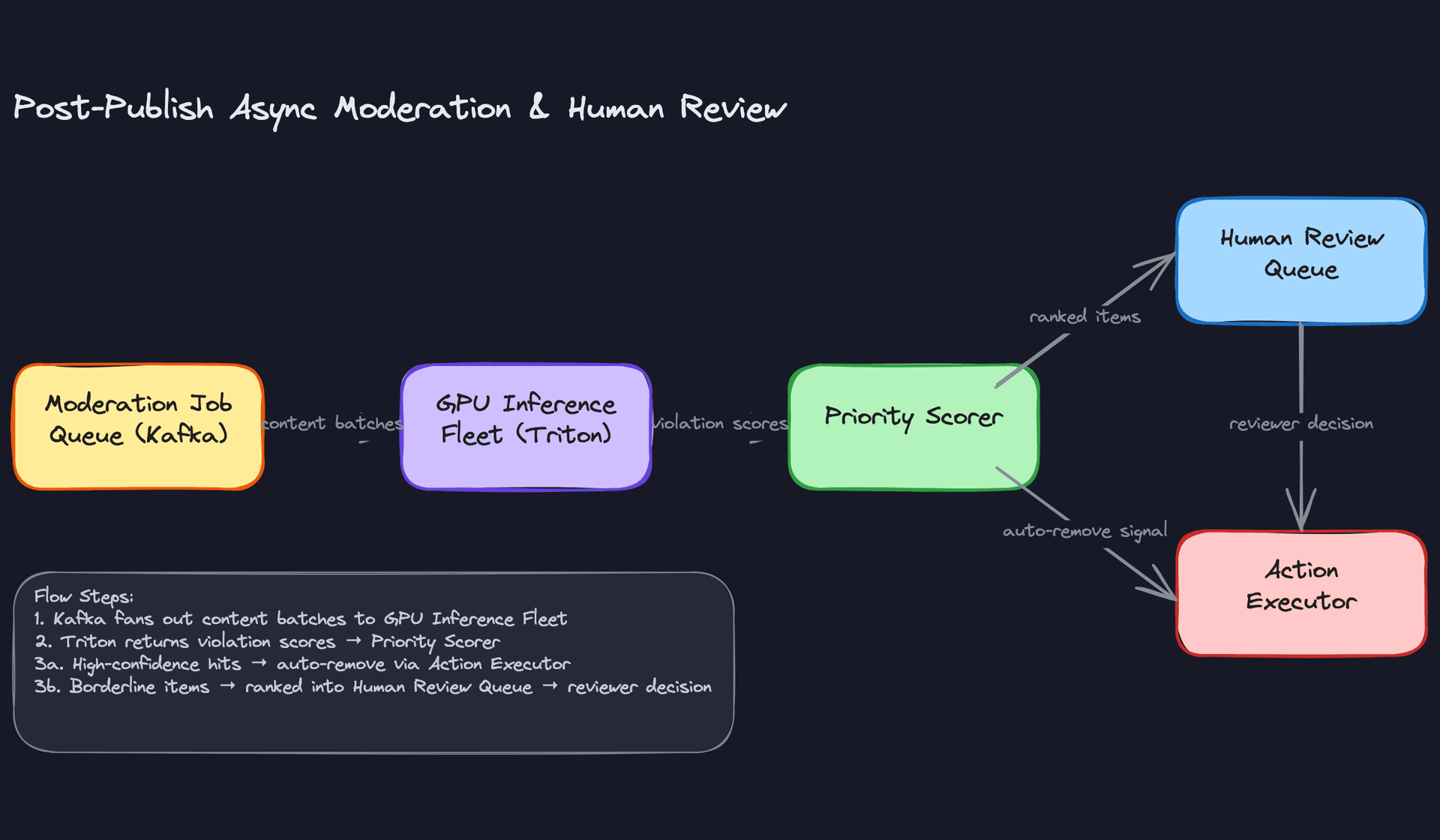
- Async post-publish review: A full multi-modal model (text + image + video frames) runs asynchronously on all content after publish, feeding a prioritized human review queue ranked by severity and virality.
- Multi-label classification: The model outputs per-category violation scores across at least four top-level categories (hate speech, NSFW imagery, spam, misinformation), not a single binary label.
- Confidence-based action routing: Model scores map to three buckets: auto-remove (high confidence), escalate to human (medium confidence or high-severity category), and auto-pass (low confidence). Thresholds are configurable per category.
- Multilingual support: The system must handle content in 50+ languages without separate per-language models.
Below the line (out of scope)
- Real-time audio moderation for live streams (separate latency and infrastructure constraints).
- Proactive detection of coordinated inauthentic behavior across accounts (a graph-level problem, not a per-item classification problem).
- Automated appeals processing for users who dispute removal decisions.
Metrics
Offline metrics
Use AUC-PR (area under the precision-recall curve) as the primary offline metric, not AUC-ROC. Because violating content is rare (well under 1% of traffic), AUC-ROC can look great even when your model misses most violations. AUC-PR is sensitive to performance on the minority class, which is exactly what you care about.
Track per-category recall at fixed precision as your operational metric. For CSAM, you might target 99.5% recall at 80% precision. For borderline political speech, you might target 90% precision at 70% recall. A single aggregate metric hides these tradeoffs.
Calibration error (expected calibration error, ECE) matters here because you are using raw model scores to route decisions. A model with good AUC but poor calibration will send the wrong items to human review.
Online metrics
- Time-to-removal for violating content (median and p95), measured from first user report or first model flag.
- False positive rate on content from high-reach accounts, tracked separately because wrongful removals there generate disproportionate trust damage.
- Human reviewer overturn rate: the fraction of model-escalated items that reviewers mark as non-violating. A rising overturn rate is your earliest signal that the model is degrading.
Guardrail metrics
- Pre-publish path p99 latency must stay under 100ms. If a model update pushes this above threshold, it does not ship.
- Demographic fairness: false positive rates should not differ significantly across languages or demographic groups. A model that over-removes content in Arabic while under-removing it in English is a policy and legal problem.
- Human review queue depth: if the queue grows faster than reviewers can process it, auto-escalation thresholds need adjustment.
Tip: Always distinguish offline evaluation metrics from online business metrics. Interviewers want to see you understand that a model with great AUC can still fail in production. A common failure mode here is a well-calibrated model that gets gamed by adversarial users within days of deployment because it was never tested against obfuscation tactics.
Constraints & Scale
500 million pieces of content per day works out to roughly 5,800 items per second on average, with peak traffic around 10,000 QPS. That peak is what you design for.
The pre-publish path is the hard constraint. You have a synchronous call in the upload critical path, which means your fast classifier needs to run on CPU (no GPU cold-start latency) and finish in under 50ms to leave headroom for the rest of the upload flow. The async post-publish path has no hard latency SLO but does have a throughput requirement: you need to process the full day's content within a few hours to keep the human review queue fresh.
| Metric | Estimate |
|---|---|
| Prediction QPS (peak) | 10,000 QPS |
| Training data size | ~500M labeled examples (accumulated over years; active set ~50M) |
| Pre-publish inference latency budget | <50ms p99 (CPU, distilled model) |
| Post-publish inference latency budget | <5s p99 (GPU, full multi-modal model) |
| Feature freshness requirement | Account behavioral signals: <60s; content embeddings: computed at upload time |
| Model size (fast path) | <200MB (must fit in CPU inference pod without large memory overhead) |
One constraint candidates often miss: the model is not stateless with respect to time. A post that gets 10 views is low priority. The same post that goes viral two hours later needs to jump to the top of the review queue. Your system needs to re-score or re-prioritize content as its reach changes, not just at the moment of upload.
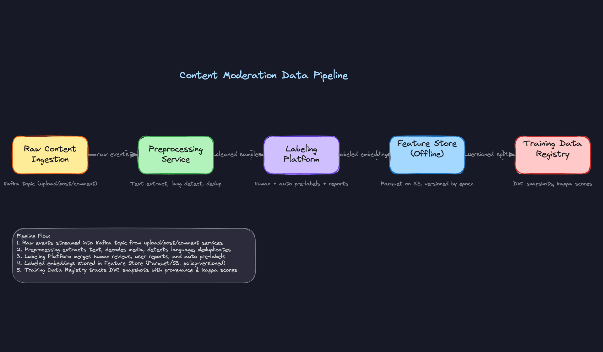
Data Preparation
Getting data right for content moderation is harder than it looks. You're not training on a clean, balanced dataset of cat photos. You're working with rare, disturbing, legally sensitive content that users and adversaries are actively trying to hide from you. The data decisions you make here will constrain everything downstream.
Data Sources
You have four main signals to work with, and each has a different reliability profile.
User reports are your highest-recall source for novel violations. When something goes viral and wrong, reports spike before your models catch it. The problem is precision: users report content they simply dislike, not just content that violates policy. Expect 60-70% of reports to be non-actionable on most platforms. Volume is high (tens of millions per day at scale), but you need to treat reports as weak labels, not ground truth.
Proactive detection signals come from your existing classifiers, hash-matching systems, and rule-based filters running continuously on all content. These generate candidate violations without waiting for user reports. They're biased toward patterns your current models already know, which is exactly the blind spot you need to worry about.
Human reviewer decisions are your gold standard. Reviewers working from a policy guide produce the highest-quality labels you'll get. The catch: volume is limited (a reviewer might process 200-400 items per shift), and reviewer decisions themselves have noise. Reviewers disagree, especially on borderline cases.
Synthetic adversarial examples are underrated. Your red team generates content designed to evade your classifiers: misspelled slurs, images with text overlaid, videos with policy-violating audio but benign frames. Without these, your model will be brittle against even basic evasion attempts. Generate them deliberately and include them in training.
Interview tip: When the interviewer asks about data sources, don't just list them. Immediately follow up with the reliability and bias profile of each. That's the signal that separates candidates who've thought about this from those who haven't.
For event logging, every piece of content that enters the system should emit a structured event at upload time:
{
  "content_id": "uuid",
  "user_id": "uuid",
  "content_type": "text|image|video",
  "modalities_present": ["text", "image"],
  "language": "en",
  "upload_timestamp": "2024-01-15T14:23:01Z",
  "account_age_days": 142,
  "prior_violations_30d": 0,
  "surface": "post|comment|dm|story"
}
Capture the surface (post vs. DM vs. comment) from day one. Violation rates and policy thresholds differ significantly by surface, and you'll want to train surface-specific models later.
Label Generation
The label schema matters as much as the labels themselves. A flat binary "safe/unsafe" label is useless in production. You need a hierarchical taxonomy:
Hate Speech
  └── Targeted harassment (severity: high)
  └── Slurs without targeting (severity: medium)
  └── Coded language / dog whistles (severity: medium)
NSFW
  └── CSAM (severity: critical, auto-escalate)
  └── Non-consensual intimate imagery (severity: high)
  └── Graphic violence (severity: high)
Spam
  └── Coordinated inauthentic behavior (severity: high)
  └── Commercial spam (severity: low)
Each piece of content gets a multi-label annotation, not a single category. A post can be both hate speech and spam (coordinated harassment campaigns are common). Your model needs to output a score per leaf node, not pick one winner.
For inter-annotator agreement, track Fleiss' kappa per category. Anything below 0.6 is a signal that your policy definition is ambiguous, not that your reviewers are bad. When kappa is low on a category, go back to the policy team before you collect more labels. More labels on a broken definition just gives you more noise.
Warning: Label leakage is one of the most common ML system design mistakes. Always clarify the temporal boundary between features and labels. In content moderation, this means your training features must only include signals available at the moment of upload. Reviewer decisions made three days later cannot be used as features, only as labels.
The label generation pipeline looks like this: a piece of content enters the review queue, a reviewer makes a decision using the policy guide, that decision is recorded with the reviewer ID and timestamp, and a separate adjudication step resolves disagreements when two reviewers conflict. Only adjudicated decisions graduate to training labels.
For implicit signals, watch-time and engagement are weak proxies for safety. High engagement on violating content is common (outrage drives clicks). Don't use engagement as a positive label. User reports are better, but still noisy. Treat them as a signal to prioritize human review, not as a label directly.
Data Processing & Splits
Deduplication is non-negotiable. Coordinated campaigns repost identical or near-identical content at scale. If you don't deduplicate before splitting, the same content appears in train and test, and your eval metrics are meaningless. Use perceptual hashing for images and SimHash for text to catch near-duplicates, not just exact matches.
Bot filtering comes next. A significant fraction of policy-violating content comes from automated accounts. If bot-generated content dominates your training set, your model learns to detect bots, not violations. Filter by account signals (account age, posting velocity, device fingerprint) before training.
The class imbalance problem here is severe. Violating content is typically under 1% of all traffic. A model that predicts "safe" for everything gets 99%+ accuracy and is completely useless. Three strategies work together:
Stratified sampling ensures each training batch has a minimum representation of each violation category. Hard negative mining pulls in near-miss examples: content that looks like a violation but isn't, or content that evaded detection until a human caught it. These are the most informative negatives you have. Oversampling minority classes (especially rare but critical categories like CSAM) prevents the model from treating them as statistical noise.
For train/val/test splits, never split randomly. Content moderation has strong temporal patterns. Adversarial tactics evolve, policy definitions change, and new content formats emerge. A random split leaks future patterns into training and makes your offline metrics far more optimistic than your production performance will be.
Split by time: train on everything before month N, validate on month N, test on month N+1. This mirrors the actual deployment scenario where your model always predicts on content it hasn't seen yet.
Data versioning is where most teams cut corners and regret it. When your policy team updates the definition of "coordinated inauthentic behavior," you need to retroactively re-label six months of historical data. If you don't have lineage tracking, you can't do that safely. Use DVC or Delta Lake to snapshot your training datasets with the policy version, label schema version, and annotator pool metadata attached. Every model in MLflow should trace back to an exact dataset snapshot. When something goes wrong in production, you need to answer "which data trained this model" in minutes, not days.
Key insight: Policy definitions change more often than you expect. At Meta or YouTube, policy updates happen multiple times per year. Your data infrastructure needs to support retroactive re-labeling as a first-class operation, not an emergency procedure.
Raw violating content, especially CSAM, cannot live in your standard data lake. It must sit in restricted-access storage with role-based access controls, access audit logs, and strict retention limits (often mandated by law). Your training pipeline reads hashes and embeddings from this content, not the raw bytes. PhotoDNA handles perceptual hashing for CSAM specifically and is the industry standard. Any engineer who needs to access raw violating content for debugging goes through an approval workflow, and that access is logged. Design this from day one; retrofitting access controls onto a data lake is painful.
Feature Engineering
Content moderation pulls from three very different signal sources: the content itself (text, pixels, audio), the account that posted it, and the behavioral context around the submission. Getting these features right matters more than model architecture. A well-calibrated classifier on good features will outperform a transformer on garbage inputs every time.
Feature Categories
Content Features (Text)
The text in a post is your richest signal, but raw tokens aren't enough. You need semantic representations that generalize across languages and evolve with adversarial evasion tactics like leetspeak, zero-width characters, and deliberate misspellings.
| Feature | Type | How It's Computed |
|---|---|---|
| Multilingual sentence embedding | float[768] | XLM-RoBERTa CLS token, fine-tuned on policy-labeled data |
| N-gram toxicity score | float | TF-IDF over known slur/threat n-gram vocabulary, normalized |
| URL reputation score | float | Lookup against Safe Browsing API + internal domain blocklist |
| OCR text embedding | float[768] | Tesseract or Google Vision OCR output fed into same text encoder |
| Language ID | categorical | fastText language classifier, one-hot or embedding |
The OCR feature is one most candidates forget. A huge fraction of policy-violating text arrives as an image of text, specifically to evade text classifiers.
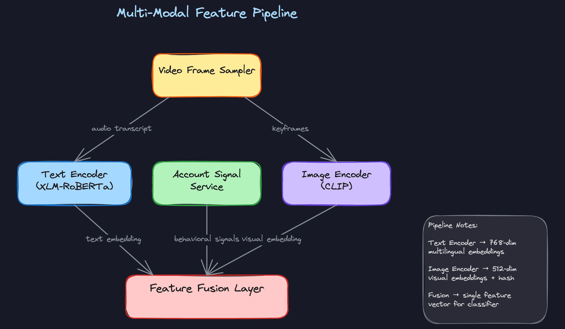
Content Features (Image and Video)
Image features split into two jobs: matching known-bad content and detecting novel violations.
For known-bad matching, perceptual hashing (pHash or PhotoDNA for CSAM) gives you an exact-ish lookup against a blocklist database. This runs in microseconds and catches re-uploaded known violations before any model touches the content.
For novel detection, CLIP embeddings are your workhorse. A 512-dim CLIP visual embedding lets you do zero-shot category detection ("does this image look like a weapon?") and nearest-neighbor search against labeled examples. You can also run a dedicated object detection model (YOLO or a fine-tuned ViT) that outputs structured signals: nudity region confidence, weapon presence, gore score. These structured outputs are easier to threshold and audit than raw embeddings.
Video adds a temporal dimension. You can't run the full image pipeline on every frame at 10K QPS. The practical approach is scene-change-triggered keyframe extraction: sample densely when the visual content changes significantly, sparsely otherwise. Each keyframe feeds the image pipeline. Audio gets transcribed via Whisper and routed directly into the text pipeline. At the end, you aggregate per-frame violation scores (max, mean, and 90th percentile) as three separate features, because a single violent frame in an otherwise benign video is a very different signal than sustained violent content.
Account and Behavioral Features
These features don't describe the content at all. They describe the entity posting it, and they're often the fastest signal you have.
| Feature | Type | How It's Computed |
|---|---|---|
| Account age (days) | int | now() - account_created_at |
| Prior violation count (90d) | int | Aggregated from moderation action log, batch-updated daily |
| Post frequency (24h) | float | Rolling count from Kafka event stream, updated every 5 min |
| Violation rate (30d) | float | violations_30d / posts_30d, batch-computed |
| Session velocity | float | Posts-per-minute in current session, computed at request time |
A brand-new account posting at 200 posts per minute with two prior violations in the last week is almost certainly a spam or coordinated inauthentic behavior campaign. The model doesn't need to read the content to assign a high prior probability of violation.
Cross-Modal and Interaction Features
Late in the pipeline, after you have embeddings from each modality, you construct cross-modal features. The simplest version is cosine similarity between the text embedding and the image embedding. A post where the caption says "beautiful sunset" but the image embedding is closest to known NSFW content is a strong signal of intentional mislabeling.
You can also compute account-category affinity: how often has this account historically posted content that was flagged in each violation category? This is a sparse feature (most accounts have zero history in most categories), so represent it as a float vector over your category taxonomy rather than one-hot.
Feature Computation
Different features have very different freshness requirements, and that drives three separate computation paths.
Batch Features
Account age, 30-day violation rate, and prior violation counts don't need to be current to the second. A daily Spark job reads from the moderation action log and user table, computes aggregates, and writes results to the offline feature store as Parquet on S3. A separate job then pushes the latest values into Redis for online serving.
# PySpark batch job: compute per-account violation features
from pyspark.sql import functions as F

violation_features = (
    moderation_actions
    .filter(F.col("action_date") >= F.date_sub(F.current_date(), 30))
    .groupBy("account_id")
    .agg(
        F.count("*").alias("violation_count_30d"),
        F.countDistinct("category").alias("distinct_categories_30d"),
        F.max("severity").alias("max_severity_30d")
    )
)

# Write to offline store
violation_features.write.parquet("s3://feature-store/account_violations/dt=2024-01-15/")
The offline store snapshot is what your training jobs read. This is important: when you train a model in February on data from January, you need the feature values as they existed in January, not today's values. Partition by date and always join training examples to the feature snapshot from the same time window.
Near-Real-Time Features
Post frequency and session velocity can't wait for a daily batch job. A spike in posting rate is a signal that needs to be visible within minutes, not the next morning.
The pipeline here is Kafka to Flink to Redis. The Flink job maintains a sliding window count per account and writes updated values to Redis with a TTL. At inference time, the feature server reads from Redis.
# Flink streaming job: rolling post count per account (pseudocode)
env = StreamExecutionEnvironment.get_execution_environment()

post_stream = (
    env
    .add_source(KafkaSource("content_submissions"))
    .key_by(lambda e: e["account_id"])
    .window(SlidingEventTimeWindows.of(Time.hours(24), Time.minutes(5)))
    .aggregate(CountAggregate())
)

post_stream.add_sink(RedisSink(key_pattern="feat:post_freq_24h:{account_id}"))
The 5-minute slide means your feature is at most 5 minutes stale. For spam detection, that's acceptable. For something like session velocity (posts per minute in the current session), you'd tighten the window to 1 minute.
Real-Time Features
Text and image embeddings for new content can't be precomputed because the content doesn't exist yet. These get computed at request time, inline in the serving path.
For the synchronous pre-publish path, this means the embedding computation is part of your latency budget. XLM-RoBERTa on CPU takes ~80-120ms for a typical post. That's why the pre-publish path uses a distilled model (covered in the serving section). For the async post-publish path, you have more headroom and can run the full encoder on GPU.
One optimization: if the same image gets re-uploaded (common with viral content and spam campaigns), cache the CLIP embedding keyed on the perceptual hash. The first upload pays the encoding cost; every subsequent re-upload is a Redis lookup.
Feature Store Architecture
The feature store has two layers that serve different masters.
The offline store (Parquet on S3, queryable via Hive or Spark) is for training. It's append-only, partitioned by date, and stores the full history of feature values. When you kick off a training run, you join your labeled examples to the offline store using a point-in-time join: for each training example with a timestamp t, you fetch the feature values that were available at time t. This is non-negotiable. Joining to today's feature values when training on historical examples is a form of data leakage that will make your offline metrics look better than your online metrics.
The online store (Redis) is for serving. It holds only the latest value per entity, with TTLs to prevent stale data from accumulating. The feature server reads from Redis with a target p99 of under 5ms.
Key insight: The most common failure mode in ML systems is training-serving skew. Features computed differently in batch training versus online serving will silently degrade your model. The fix is to share computation logic: define features once in a framework like Feast, and let it generate both the Spark batch job and the Redis serving path from the same definition. If you can't do that, at minimum write integration tests that run the batch and online computation on the same input and assert the outputs match.
The skew problem is especially sharp for content moderation because your features span three computation paths (batch, streaming, real-time) and two modalities with different preprocessing steps. A common bug: the batch job normalizes image embeddings to unit length, but the online encoder doesn't. Your cosine similarities in training look great. In production, they're garbage. Test this explicitly before every model launch.
Model Selection & Training
Model Architecture
Start simple. Before you touch a GPU, your baseline should be a fine-tuned XLM-RoBERTa with a sigmoid multi-label head. One model, one forward pass, outputs a probability per violation category. This gives you calibrated precision/recall curves per category that every future architecture has to beat. Interviewers love when you anchor the conversation in a concrete benchmark rather than jumping straight to the fancy stuff.
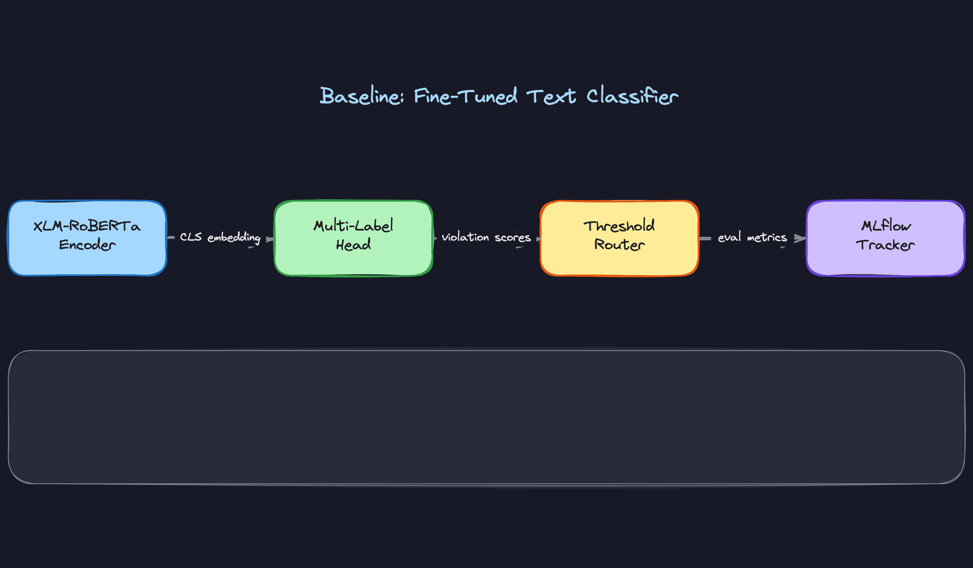
The input/output contract for the baseline:
# Input
{
  "text": str,                  # raw post text, up to 512 tokens
  "lang": str,                  # ISO 639-1 language code (e.g., "en", "ar")
}

# Output
{
  "scores": {
    "hate_speech": float,       # [0, 1] sigmoid probability
    "nsfw": float,
    "spam": float,
    "misinformation": float,
    "csam": float,
  },
  "model_version": str,
  "latency_ms": float
}
XLM-RoBERTa earns its place here because you're operating across 50+ languages and you can't afford separate models per locale. The CLS token embedding captures cross-lingual semantics out of the box. Binary cross-entropy loss per label, summed across categories, fits the multi-label objective cleanly since violation categories aren't mutually exclusive (a post can be both spam and hate speech).
Once the baseline is solid, you upgrade to the production architecture: separate encoders per modality feeding a late-fusion MLP.
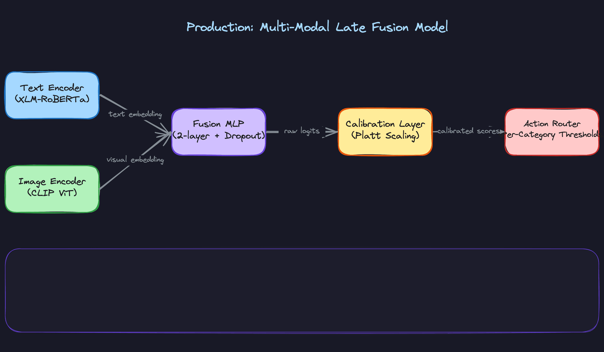
Late fusion wins over early fusion here for a practical reason: when policy changes, you can retrain just the text encoder without touching the image encoder, and vice versa. Early fusion tangles the modalities together and makes debugging misclassifications much harder. The fusion MLP is two layers with dropout, sitting on top of concatenated embeddings from text (768-dim from XLM-RoBERTa) and image (512-dim from CLIP ViT-L/14).
Missing modalities are a real problem at inference time. A text-only post has no image embedding. Don't crash; substitute a learned zero vector that the MLP was trained to handle. During training, randomly drop modalities with 20% probability per sample so the model learns to be robust to this.
def fuse_embeddings(text_emb, image_emb, modality_mask):
    # modality_mask: [has_text, has_image]
    text_emb  = text_emb  * modality_mask[0]   # zero-out if missing
    image_emb = image_emb * modality_mask[1]
    fused = torch.cat([text_emb, image_emb], dim=-1)  # (B, 1280)
    return fused
Threshold Calibration
Raw sigmoid outputs are not calibrated probabilities. A score of 0.7 doesn't mean there's a 70% chance this content violates policy, especially after fine-tuning on imbalanced data. Before you wire model scores to actions, run Platt scaling or isotonic regression on a held-out calibration set.
Each category gets its own threshold, and each threshold maps to one of three action buckets:
| Score range (post-calibration) | Action |
|---|---|
| Above auto-remove threshold | Auto-remove, log for audit |
| Between thresholds | Escalate to human review queue |
| Below auto-pass threshold | Pass, sample for monitoring |
The thresholds are not symmetric across categories. For CSAM, you set recall at 99.9%+ and accept a higher false positive rate. For borderline political speech, you flip that: err toward precision and send more to human review rather than auto-removing. This is a policy decision, not a modeling decision, but you need to make it explicit in your design.
Tip: When an interviewer asks "how do you choose thresholds," don't say "we tune them on validation." Walk through the business logic: who bears the cost of a false positive (wrongly removed content) vs. a false negative (missed violation)? The answer differs by category, and that's what drives the threshold asymmetry.
Training Pipeline
Distributed fine-tuning runs on 8xA100 nodes using DeepSpeed ZeRO-3. ZeRO-3 shards optimizer states, gradients, and model parameters across all GPUs, which lets you fit XLM-RoBERTa plus the fusion layers in memory without gradient accumulation hacks. Mixed precision (bf16) and gradient checkpointing cut memory further at a small compute cost.
# DeepSpeed config (abbreviated)
zero_optimization:
  stage: 3
  offload_optimizer:
    device: cpu
bf16:
  enabled: true
gradient_checkpointing: true
train_micro_batch_size_per_gpu: 32
Every experiment logs to Weights & Biases: per-category AUC-PR, precision at fixed recall thresholds, calibration error, and GPU utilization. AUC-PR matters more than AUC-ROC here because your class distribution is severely imbalanced (violating content is under 1% of traffic). A model that flags nothing still gets 99% accuracy. AUC-PR punishes that.
Retraining schedule. Full retraining weekly, triggered by a cron job against the latest versioned dataset snapshot. Incremental fine-tuning (continuing from the last checkpoint on new data only) runs daily for fast adaptation to emerging abuse patterns. The risk with incremental-only is catastrophic forgetting: the model drifts away from older violation types that aren't appearing in fresh data. Weekly full retraining is your insurance policy against that.
Data windowing. Use a rolling 90-day window for the main training set, with a fixed 30-day holdout for evaluation. Older data is downweighted by a time decay factor rather than dropped entirely, since some violation patterns are stable across time. When policy changes, the window resets to the policy effective date to avoid training on labels that no longer reflect current rules.
Hyperparameter tuning. Bayesian optimization via Optuna over learning rate, warmup steps, and fusion MLP hidden size. You're not doing a full grid search on a model this size; three to five trials with early stopping based on validation AUC-PR is enough to find a good configuration. Lock the transformer backbone learning rate an order of magnitude lower than the fusion head (1e-5 vs. 1e-4) to avoid catastrophic forgetting of pretrained representations.
Offline Evaluation
AUC-PR per category is your primary metric. But before you call a model ready to ship, you need three more checks.
Calibration. Plot a reliability diagram: if the model says 0.8, does it violate policy 80% of the time in the holdout set? Poorly calibrated models make threshold-setting unreliable. Expected Calibration Error (ECE) below 0.05 is a reasonable bar.
Fairness slices. Evaluate precision and recall broken out by language, content type, and account age. Models trained on English-heavy data routinely underperform on Arabic or Hindi content. If recall on non-English content is 15 points lower than English, that's a deployment blocker, not a footnote.
Error analysis. Sample 200 false positives and 200 false negatives per category and read them. This sounds tedious; it's the most valuable hour you'll spend before launch. False positives in the hate speech category often cluster around counter-speech (quoting a slur to condemn it) and satire. False negatives cluster around coded language and dog whistles that weren't in training data. These patterns tell you exactly what to prioritize in your next labeling sprint.
Common mistake: Candidates report a single AUC number and move on. Interviewers at Meta or YouTube will push back immediately: "What's your recall on Arabic content?" "What happens to precision when a new slang term goes viral?" Have answers for those questions, or at least a framework for how you'd find them.
Backtesting. For policy changes, time-based backtesting matters more than random holdout splits. Train on data before a known policy update, evaluate on data after it, and measure how much performance degrades. This simulates the real deployment scenario where the model was trained before the world changed.
Policy Change Adaptation
When policy definitions shift (say, the platform adds new rules around AI-generated synthetic media), you have two options: full retraining from scratch on re-labeled data, or continual learning from the last checkpoint.
Full retraining is safer but slow. Continual learning is faster but risks forgetting. The practical answer is both: use continual learning to deploy a fast-adapted model within 48 hours of a policy change, then replace it with a fully retrained model two weeks later once re-labeling is complete.
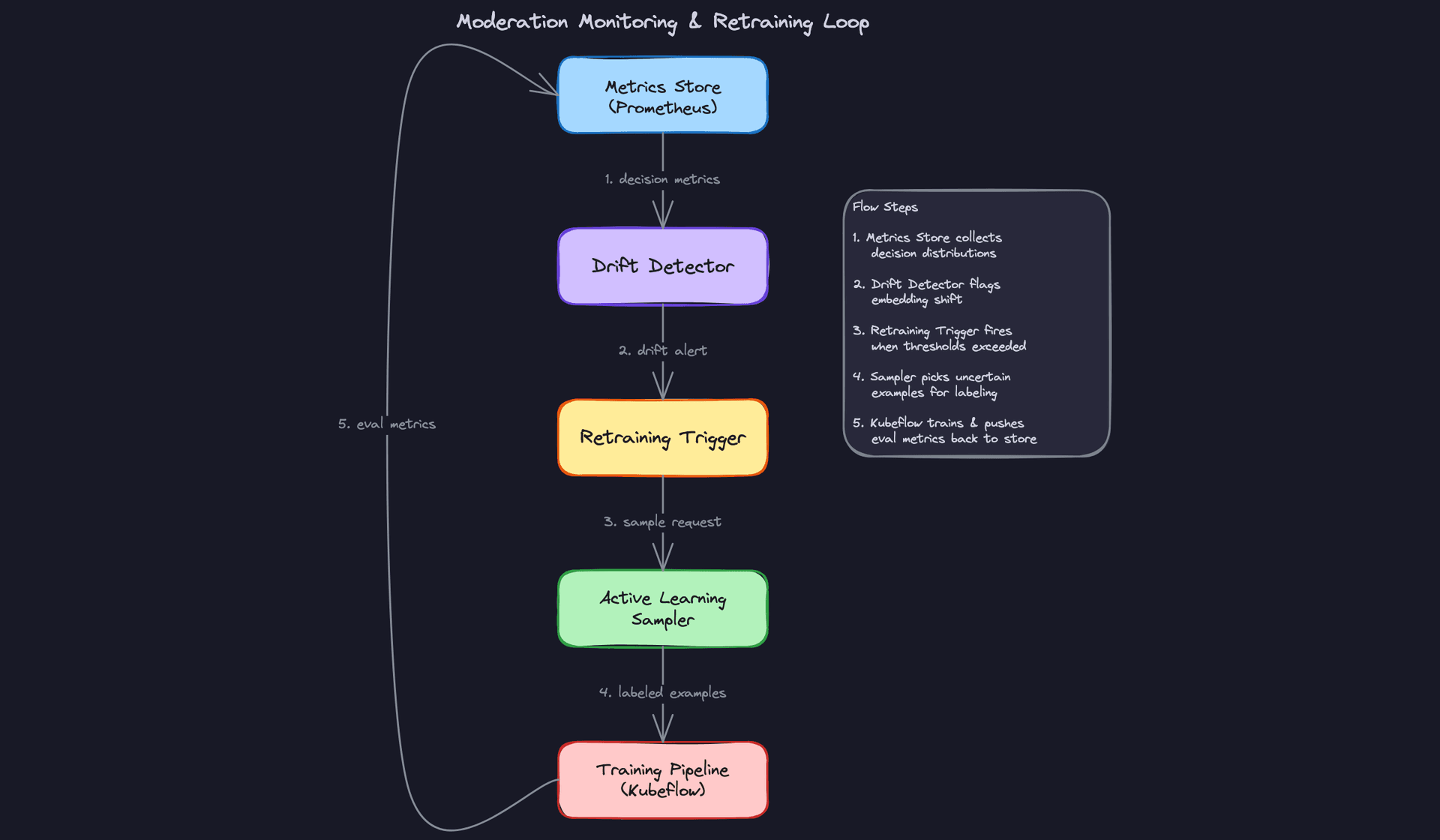
Active learning makes the re-labeling budget go further. Rather than randomly sampling content for human reviewers to label, rank examples by model uncertainty (entropy of the output distribution) and by expected impact (high-virality content where a wrong decision matters more). Reviewers spend their time on the examples that will move the model the most.
def active_learning_score(entropy: float, virality_rank: float) -> float:
    # entropy: model uncertainty [0, log(n_classes)]
    # virality_rank: normalized [0, 1], higher = more viral
    return 0.6 * entropy + 0.4 * virality_rank
This score feeds directly into the human review queue priority, so the labeling pipeline and the reviewer workflow share the same infrastructure. That's the kind of system-level thinking that separates a senior answer from a mid-level one.
Inference & Serving
Content moderation is one of the few ML systems that genuinely needs both online and batch inference running simultaneously, for different reasons. Get the architecture wrong and you're either blocking users with 500ms latency spikes or letting violating content sit live for hours while your GPU queue backs up.
Serving Architecture
The core insight is that you have two fundamentally different latency budgets depending on when moderation happens.
Pre-publish means the user is waiting. They hit "post," and your system has to decide before writing to the database. That's a hard wall around 100ms end-to-end, which leaves maybe 50ms for the model itself after you account for network, feature fetch, and serialization overhead.
Post-publish means the content is already live. Latency still matters for limiting harm, but you're optimizing for throughput and accuracy, not raw speed. A few seconds is acceptable. A few minutes is not.
This naturally maps to two separate serving paths:
- Synchronous path: distilled CPU-based classifier, called inline during the upload request
- Asynchronous path: full multi-modal fusion model on a GPU fleet, consuming from a Kafka topic
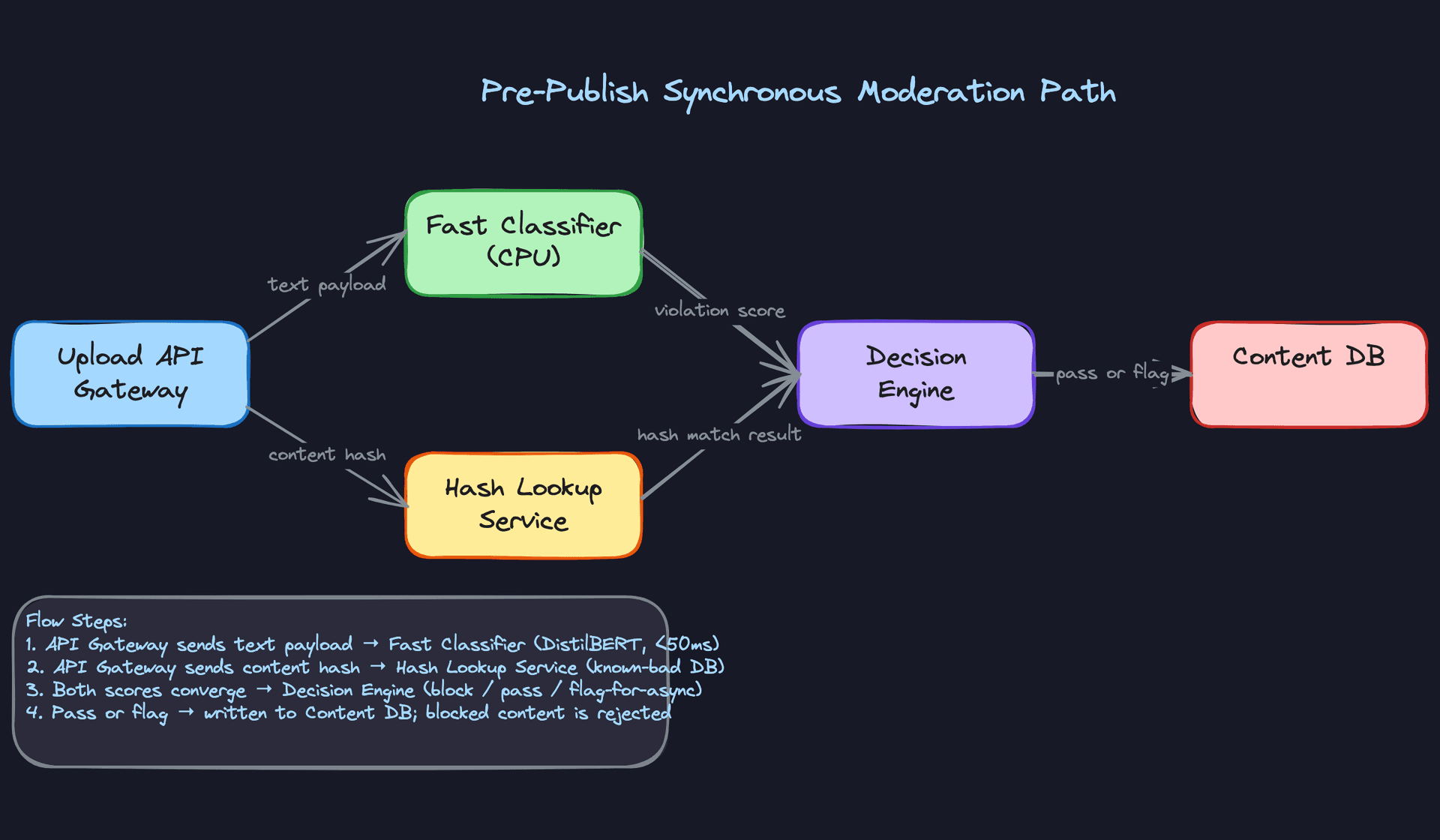
The synchronous path runs a distilled DistilBERT model alongside a perceptual hash lookup. The hash check is nearly free and catches known-bad content (CSAM, recycled spam) instantly. The classifier handles everything else. Only high-confidence violations get blocked at this stage; borderline scores pass through and get enqueued for async review. This is intentional. A false positive at pre-publish means a user's content was silently rejected, which is a trust and legal problem.
The async path is where the real work happens. Triton Inference Server runs the full multi-modal fusion model on A10G GPUs, batching requests from Kafka partitions grouped by content type. Text-only posts, image posts, and video all hit different model paths before merging at the fusion layer.
End-to-end latency breakdown for the synchronous path:
| Stage | Budget |
|---|---|
| Feature fetch (account signals from Redis) | ~5ms |
| Hash lookup | ~2ms |
| Distilled model inference (CPU) | ~30ms |
| Post-processing + threshold routing | ~3ms |
| Network + serialization overhead | ~10ms |
| Total p99 target | <50ms |
The async path has no strict per-request budget, but queue depth is your proxy metric. If the Kafka consumer lag grows, content is sitting live longer than your policy allows.
Key insight: The deployment pipeline is where most ML projects fail in practice. A model that can't be safely deployed and rolled back is a model that won't ship.
Optimization
The synchronous path lives or dies on the distilled model. Knowledge distillation from the large fusion model down to a DistilBERT-based text classifier costs roughly 3% recall on borderline categories. That's an acceptable tradeoff when the alternative is adding 400ms to every upload request. The distilled model runs on CPU, which also means you can scale it horizontally with standard web infrastructure instead of managing GPU capacity on the hot path.
For the async GPU path, the main lever is dynamic batching. Triton's built-in dynamic batching collects requests arriving within a configurable window (typically 5-20ms) and processes them together. On a single A10G, batching 32 requests at once gives you roughly 8x better throughput than processing them sequentially, with minimal latency increase since these requests are already decoupled from user-facing response time.
A few other optimizations worth mentioning in your interview:
INT8 quantization on the GPU models cuts memory bandwidth by 2x and speeds up inference ~30-40% with negligible accuracy loss on classification heads. TensorRT handles this automatically if you're deploying through Triton.
Embedding caching for the image path. CLIP embeddings for a given image are deterministic, so you can cache them in Redis keyed by content hash. Re-uploaded content (spam campaigns often reuse images) gets free inference on the image modality.
Fallback behavior matters more than most candidates discuss. If the distilled model is unavailable (deployment in progress, pod crash), you have three options: fail open (pass all content), fail closed (block all content), or fall back to hash-only detection. For most categories, fail open with aggressive async review is correct. For CSAM, fail closed is the only acceptable policy. Your decision engine needs to know which category it's operating in.
Common mistake: Candidates design a single fallback strategy for the whole system. Different content categories have different risk profiles. CSAM and child safety content requires fail-closed behavior. Spam can tolerate fail-open. Design your fallback logic per category, not per system.
Online Evaluation & A/B Testing
Shadow scoring is your first gate before any live traffic sees a new model. You deploy the candidate model alongside production, route every request to both, and log the candidate's decisions without acting on them. After 24-48 hours of shadow traffic, you compare decision divergence: what percentage of cases did the new model decide differently from production? High divergence isn't automatically bad, but it tells you where to focus your review.
For actual A/B testing, you split traffic at the content level, not the user level. Moderation decisions need to be consistent for a given piece of content regardless of who's viewing it, so you hash on content ID to assign treatment. A 5% canary is a reasonable starting point.
The metrics you track during a ramp:
- Auto-action rate per category: a sudden spike means the new model is more aggressive; a drop means it's more permissive
- Human reviewer overturn rate: reviewers overturning model decisions at a higher rate than baseline is a strong signal of regression
- False positive rate on a held-out clean content sample: you should have a golden set of known-safe content that you score on every deployment
- Latency p99: model changes can affect inference time, especially if you've changed the architecture
Statistical significance for moderation systems is tricky because violation rates are low. You're often working with rare events, which means you need longer experiment windows or you'll make decisions on noise. Two weeks of shadow data is usually the minimum before you can trust recall estimates on low-frequency categories like graphic violence.
Interleaving experiments don't apply here. That technique is for ranking systems where you want to compare two orderings in the same session. Moderation is a classification decision, not a ranking, so standard traffic splitting is the right approach.
Deployment Pipeline
Every model version goes through the same gate sequence before it touches production traffic.
Offline validation runs first. The candidate model is evaluated against a held-out reviewer-labeled test set. You're checking precision/recall per category against the current production baseline. Any category where recall drops more than 1% is a hard block. False positive rate on clean content is a separate gate with its own threshold.
REGRESSION_GATES = {
    "hate_speech":    {"min_recall": 0.92, "max_fpr": 0.02},
    "csam":           {"min_recall": 0.999, "max_fpr": 0.001},
    "spam":           {"min_recall": 0.85, "max_fpr": 0.05},
    "graphic_violence": {"min_recall": 0.88, "max_fpr": 0.03},
}
If any gate fails, the pipeline stops and alerts the team. No human override for CSAM recall gates.
Shadow deployment comes next. The model runs on 100% of traffic but takes no actions. You're collecting real-world decision distributions and comparing against production. This phase typically runs 48 hours.
Canary rollout starts at 1% of traffic taking live actions, then 5%, 10%, 25%, 50%, 100%. Each step has a minimum soak time (usually 6 hours) and automated rollback triggers:
- Auto-action rate in any category deviates more than 15% from baseline
- p99 latency on the sync path exceeds 80ms
- Reviewer overturn rate increases more than 2 percentage points
Rollback is a single config change pointing the serving infrastructure back to the previous model version. Because you're using Triton with versioned model repositories, the previous version is still loaded in memory. Rollback takes under 30 seconds.
Tip: When the interviewer asks about rollback, be specific about the mechanism. "We roll back" is not an answer. "We maintain the previous model version in Triton's model repository and flip a feature flag in the decision engine to route to version N-1" is an answer.
The canary and shadow steps are where most teams cut corners under pressure. A policy incident happens, leadership wants the new model live immediately, and the shadow phase gets skipped. That's how you end up with a model that performs well on your test set but behaves unexpectedly on the long tail of real-world content. The pipeline exists to protect you from that pressure, so build it with hard gates that require explicit override rather than soft recommendations.
Monitoring & Iteration
A content moderation system that works on launch day will fail within weeks. Adversarial users adapt, platform policy evolves, and the distribution of content shifts constantly. Monitoring isn't an afterthought here; it's the mechanism that keeps the system honest.
Tip: Staff-level candidates distinguish themselves by discussing how the system improves over time, not just how it works at launch.
Production Monitoring
Input distribution monitoring catches problems before they surface as model failures. Track the distribution of content length, language breakdown, modality mix (text-only vs. image vs. video), and account age of submitters. If the fraction of posts in a new language spikes from 2% to 15% overnight, your XLM-RoBERTa model may be operating outside its effective training distribution before a single metric degrades visibly.
Schema violations are equally important. If the upstream preprocessing service starts sending malformed embeddings or missing account-level features, your model will silently produce garbage scores. Validate feature shapes and null rates at the feature fusion layer, and alert immediately on any schema mismatch.
Model monitoring is where most teams underinvest. Prediction distribution shift is your earliest warning signal: if the fraction of content scoring above 0.8 on the hate speech head suddenly doubles, something changed. It might be a real abuse campaign, or it might be model degradation. Either way, you need to know within minutes, not days.
Measuring actual precision and recall on live traffic requires ground truth, which is the hard part. The practical approach is to sample a stratified set of model decisions daily and route them to human reviewers as a quality audit. Even a 0.1% sample at 500M items/day gives you 500K labeled examples per day. Track reviewer overturn rate per category: if reviewers are reversing more than 5% of auto-removes in a given category, that's a calibration problem.
Common mistake: Candidates track aggregate precision/recall but miss per-category degradation. A model that's 95% accurate overall can be actively harmful if it's 60% precise on political speech while being 99% precise on spam.
System monitoring covers the infrastructure layer. The metrics you need:
- Latency: p50 and p99 for both the synchronous pre-publish path and the async GPU inference fleet. A p99 spike on the sync path directly impacts upload success rates.
- GPU utilization on the Triton fleet: sustained utilization above 85% means you're one traffic spike away from queue backup.
- Human review queue depth: if the queue grows faster than reviewers can drain it, high-severity content is sitting unreviewed. Alert when queue depth exceeds a 4-hour drain time.
- Auto-action rate per category: a sudden spike in auto-removes for any category could mean a coordinated abuse campaign, or it could mean your model broke. The alert is the same; the diagnosis differs.
Alerting thresholds need to be category-aware. For CSAM, alert on any drop in recall immediately. For borderline political speech, false positive rate is the more sensitive metric and you can tolerate a slower alert cadence. Wire your alerts to PagerDuty for safety-critical categories and to Slack for quality-degradation signals that need investigation but not an immediate response.
Feedback Loops
The highest-quality training signal you have is a human reviewer overturning a model decision. That event tells you exactly where the model is wrong, on real content, with a ground-truth label. Don't waste it.
Build a pipeline that captures every overturn and routes it into a re-labeling queue. When a reviewer marks a model auto-remove as incorrect, that example should be flagged for inclusion in the next training batch with the corrected label. The pipeline looks like this: reviewer decision emitted as a Kafka event, consumed by a label ingestion service, written to your training data registry with provenance metadata (reviewer ID, timestamp, original model score, corrected label), and surfaced to the active learning sampler for prioritization.
Feedback delay is a real problem. Some signals arrive hours or days after inference. User reports, for example, accumulate over time as content spreads. Viral content that slips through pre-publish filtering may not generate enough reports to trigger review for 6-12 hours. Your monitoring pipeline needs to handle delayed label arrival without corrupting your real-time metrics.
The practical fix is to separate your evaluation windows. Use reviewer audit labels (available within hours) for fast feedback on model quality. Use user report aggregation (available over days) as a slower signal for coverage gaps, specifically content the model missed entirely. Never mix these two signals in the same precision/recall calculation; they measure different things.
Key insight: Reviewer overturn rate is a leading indicator of model drift. Embedding distribution shift (MMD against training distribution) is a lagging indicator. Use both. The overturn rate will tell you something is wrong faster than any statistical test on embeddings.
Closing the loop from alert to redeployment requires a defined runbook, not just good intentions. When the drift detector fires:
- The on-call ML engineer diagnoses whether it's input drift, model degradation, or a policy gap.
- If it's model degradation, the active learning sampler prioritizes the affected category for human review.
- Once enough labeled examples accumulate (typically 500-2K per category for fine-tuning), a retraining job triggers automatically via Kubeflow.
- The new model version runs in shadow mode against live traffic for 24 hours before promotion.
- If shadow divergence from production is within acceptable bounds and held-out metrics improve, the model promotes via canary rollout.
That full cycle should take days, not weeks. If it takes weeks, your retraining pipeline is too slow and adversarial users have already adapted.
Continuous Improvement
Retraining strategy comes down to a simple question: do you retrain on a schedule or on a trigger? The honest answer is both, for different reasons.
Scheduled retraining (weekly or biweekly) ensures the model absorbs the steady accumulation of new reviewer decisions and gradually shifting content distributions. It's low-drama and keeps the model from staling quietly. Triggered retraining fires when a specific threshold is crossed: overturn rate above 5% in a category, embedding drift score above a configured threshold, or a policy change event. Triggered retraining handles the sharp discontinuities that scheduled retraining would catch too late.
Prioritizing model improvements is where engineering judgment matters. Not every improvement is worth the same. A rough ordering:
Data quality improvements (fixing mislabeled examples, adding coverage for underrepresented languages) almost always outperform architecture changes at this stage. If your training data for Thai-language hate speech is thin, adding 10K high-quality Thai examples will beat switching from XLM-RoBERTa to a larger model every time.
Feature additions come next. Adding audio transcription from Whisper for video content, or incorporating network-level signals (coordinated posting patterns), can unlock categories of violations the per-item classifier will never catch on its own.
Architecture changes are last. They're expensive to validate, require careful A/B comparison, and the gains are often marginal once you have a well-tuned baseline with good data.
As the system matures, a few things shift. Early on, you're fighting coverage gaps: categories of violations the model has never seen. Over time, the challenge becomes adversarial robustness. Users learn what the model catches and deliberately craft content to evade it. Obfuscated text (replacing letters with lookalikes), context manipulation (embedding hate speech in otherwise benign threads), and coordinated inauthentic behavior (many accounts posting borderline content just below the threshold) all emerge as the model gets better.
At that point, per-item classification is necessary but not sufficient. You need graph-level signals: account clusters, posting velocity patterns, coordinated amplification networks. That's a different modeling problem, and it's worth flagging in the interview as the natural next evolution of the system.
Interview tip: When the interviewer asks "how would you handle adversarial users?", don't just say "retrain more often." Talk about the arms race dynamic, why per-item classifiers have a ceiling, and how network-level signals change the game. That's the answer that signals Staff-level thinking.
What is Expected at Each Level
Interviewers at different levels aren't just looking for more detail. They're looking for a fundamentally different kind of thinking. A mid-level candidate who gives a staff-level answer probably rehearsed it. A staff-level candidate who can't explain why they made each tradeoff will get caught immediately.
Mid-Level
- Design the core text classification pipeline end-to-end: ingestion, preprocessing, fine-tuned XLM-RoBERTa with a sigmoid multi-label head, and a threshold router that maps scores to actions. You don't need multi-modal at this level, but you need to own the text path completely.
- Articulate the recall vs. precision tradeoff per category. The right answer for CSAM (maximize recall, accept false positives) is the opposite of the right answer for borderline political speech (minimize false positives, accept some misses). Interviewers will probe this directly.
- Describe a basic human review queue: what goes in it, how items get prioritized, and how reviewer decisions feed back into the system. Even a simple "high-confidence violations auto-remove, everything else gets queued" answer shows you understand the human-in-the-loop design.
- Know how to explain threshold calibration. Why raw model scores aren't probabilities, and what Platt scaling does. You don't need to derive it, but you need to know why it matters when you're setting action thresholds.
Senior
- Handle multi-modal inputs and explain the late fusion architecture. More importantly, explain why late fusion: it lets you update one modality's encoder independently, debug failures per modality, and handle missing modalities gracefully at inference time.
- Design both serving paths. The synchronous pre-publish path needs a distilled CPU model under 50ms p99. The async post-publish path can use the full GPU-backed fusion model via Triton. If you conflate these two paths or design one model to serve both, that's a red flag.
- Proactively raise the feedback loop. Senior candidates don't wait to be asked "how does the model improve over time?" They bring it up when discussing the human review queue, because reviewer overturn decisions are your highest-quality training signal.
- Reason about model distillation as an explicit engineering tradeoff, not just a trick. You're accepting roughly 3% recall degradation in exchange for a 10x latency reduction. That's a product decision as much as an ML one, and you should frame it that way.
Common mistake: Senior candidates often design a great offline training pipeline and a great serving system, but leave a gap between them. The interviewer will ask "how does a reviewer decision get back into training?" If you haven't thought through that pipeline, it signals you've only built half the system.
Staff+
- Drive policy versioning as a first-class system concern. When the platform's definition of "hate speech" changes, you need to re-label historical data, retrain, and run a shadow comparison before rollout. This isn't an afterthought; it's a core part of the architecture. Staff candidates design for policy change from the start.
- Discuss concept drift and adversarial robustness together. Adversarial users don't just post bad content; they probe your classifier, find the decision boundary, and exploit it systematically. Monitoring embedding distribution shift and reviewer overturn rate gives you early warning, but you also need to think about coordinated inauthentic behavior that evades per-item classifiers entirely.
- Raise the organizational and legal tradeoffs of auto-action at scale. Wrongly removing content has real consequences: user trust, regulatory exposure, and in some jurisdictions, legal liability. Staff candidates don't just optimize for recall; they articulate who owns the decision when the model is wrong and what the appeals process looks like.
- Frame active learning as a resource allocation problem. You have a finite number of human reviewer hours. Active learning lets you direct those hours toward the examples that will most improve the model, specifically high-uncertainty items near the decision boundary and high-impact items in underrepresented categories. This is the difference between a system that improves slowly and one that adapts quickly to new abuse patterns.
Key takeaway: Content moderation isn't a classification problem with a human fallback. It's a human judgment system with a classifier to handle scale. Every design decision, from threshold calibration to queue prioritization to feedback loops, should reflect that the model exists to support human policy enforcement, not replace it.
