Problem Formulation
Before you write a single line of model code, you need to nail down what the system is actually doing. Interviewers will probe this early, and candidates who skip straight to "train a two-tower model" without clarifying the product surface almost always back themselves into a corner.
Start by asking: is this a "customers who viewed this also viewed" widget, or a "similar items" widget on the product detail page? They sound identical but they're not. The first is collaborative by nature, built on session co-occurrence. The second can be answered purely from item content, which means it works even for brand-new listings. That distinction drives your entire model architecture.
Clarifying the ML Objective
ML framing: Given a query item ID, retrieve and rank an ordered list of K items that are most similar to it, where similarity is defined by a combination of visual, textual, and behavioral signals.
This is a retrieval and ranking problem, not classification or regression. You're not predicting a label; you're embedding items into a shared vector space and finding nearest neighbors. The ranking layer on top of retrieval is lightweight, but the retrieval quality is everything.
"Success" means different things depending on who you ask. The business wants higher CTR on the similar items widget and more add-to-cart events. The ML team measures Recall@10 on held-out sessions. These are correlated but not the same. A model that maximizes visual similarity might return near-identical colorways that look great offline but frustrate users who wanted something genuinely different. You need to define success in both terms before the interview ends.
The other thing to lock down early: what does "similar" mean? Content similarity (same visual style, same category, overlapping description keywords) and behavioral similarity (users who viewed this also viewed that) capture fundamentally different signals. A red leather handbag and a brown leather handbag are content-similar. A handbag and a matching wallet are behaviorally similar. Your system probably needs both, and your model choice follows from that.
Functional Requirements
Core Requirements
- The model takes a single item ID as input and returns an ordered list of K similar items (K is typically 10 to 20, configurable per surface).
- Similarity must reflect a hybrid of content signals (image, title, category) and behavioral signals (co-view, co-purchase), with content as the fallback for new items.
- New items must appear in similarity results within 2 hours of being listed, even before any behavioral data accumulates.
- The system must enforce diversity constraints at serving time: no more than 2 results from the same brand, and no near-duplicate colorways (cosine similarity above 0.98 between two candidates should trigger deduplication).
- Results must be filtered by business rules before returning: out-of-stock items and policy-violating listings are excluded.
Below the line (out of scope)
- Personalization based on the viewing user's history. This is item-to-item similarity, not user-to-item recommendation.
- Real-time embedding updates as a user browses (session-aware retrieval is a separate system).
- Cross-catalog similarity across different product verticals (e.g., recommending a shoe to someone viewing a jacket).
Metrics
Offline metrics
Recall@10 is your primary offline metric. For each query item in your eval set, you check whether the ground-truth "similar" items (derived from co-view sessions) appear in the top 10 results. It directly measures whether your retrieval is finding the right candidates.
NDCG@10 adds position sensitivity on top of recall. If the best match is ranked 9th instead of 1st, NDCG penalizes that. Use it when you care about the ordering of results, not just set membership.
Intra-list diversity (average pairwise distance between returned items) is an offline guardrail. If this number collapses, your model is returning near-duplicate clusters, which is a real failure mode with contrastive models that overfit to visual similarity.
Cold-start Recall@10, computed separately on items with zero behavioral history, tells you whether your content-only fallback is actually working. Don't let it get averaged into your main metric and disappear.
Online metrics
CTR on the similar items widget is the primary signal. Add-to-cart rate from widget clicks is a stronger signal because it filters out curiosity clicks. Session depth (pages per session after a similar items click) tells you whether users are finding the widget genuinely useful or just bouncing.
Guardrail metrics
P99 serving latency must stay under 100ms. Catalog coverage (what percentage of items have at least one valid similar item returned) should stay above 95%. If coverage drops, something in your pipeline is silently failing.
Tip: Always distinguish offline evaluation metrics from online business metrics. Interviewers want to see you understand that a model with great AUC can still fail in production. A model with 0.85 Recall@10 that returns near-duplicate results will have lower CTR than a model with 0.78 Recall@10 that returns genuinely diverse alternatives.
Constraints & Scale
The catalog has 500 million items. At 50K QPS peak, you cannot recompute embeddings on the fly for every request. That rules out any approach where inference happens at query time for the full catalog. Your architecture must separate the embedding generation (batch, offline) from the similarity lookup (online, fast).
The 2-hour freshness SLA for new items is the hardest constraint. A nightly batch rebuild of your ANN index won't cut it. You need an incremental indexing path that can ingest new item embeddings and make them queryable within the SLA window.
| Metric | Estimate |
|---|---|
| Prediction QPS | 50,000 requests/sec at peak |
| Training data size | ~10B co-view events/month, 500M item embeddings at 256 dims (~500GB fp32) |
| Model inference latency budget | p99 < 100ms end-to-end; ANN lookup target < 20ms |
| Feature freshness requirement | New items indexed within 2 hours of listing |
The memory math matters here. 500M items at 256 dimensions in float32 is 512GB of raw vectors. You cannot fit that in RAM on a single machine. Index sharding across a CPU fleet, combined with quantization (int8 or product quantization), gets you to a manageable per-shard footprint. That's a conversation the interviewer will almost certainly push you toward, so have the numbers ready.
Data Preparation
Your system is only as good as the data feeding it. For a similar items system at 500M catalog items and 50K QPS, getting the data pipeline wrong doesn't just hurt model quality; it creates silent failures that are nearly impossible to debug in production.
Data Sources
Two fundamentally different data streams power this system, and you need both.
Item catalog data comes from your product catalog service: titles, descriptions, images, price, brand, and category taxonomy. At scale, this isn't a static dump you pull once. You need change-data-capture (CDC) on the catalog database to detect new listings, price changes, and delistings in near-real-time. A new item listed at 9am should be eligible for similarity results by 11am, not tomorrow's batch run.
Expect this data to be messy. Images are missing or corrupted for roughly 5-15% of items in any large marketplace catalog. Descriptions are truncated, duplicated across variants, or written in inconsistent languages. Category taxonomy is often misapplied by sellers. You'll need to decide upfront which of these are hard blockers (no image at all) versus soft degradations (low-res image) that still allow indexing with reduced confidence.
Behavioral event data is your co-view and co-purchase signal. Every time a user views item A and then item B in the same session, that's a weak positive pair. A purchase after viewing is a stronger signal. These events flow through Kafka at high volume; at 50K QPS on the serving side, you're likely ingesting millions of events per hour during peak traffic.
| Source | Signal | Volume | Freshness | Reliability |
|---|---|---|---|---|
| Product catalog (CDC) | Item attributes, images, taxonomy | ~500M items; tens of thousands of updates/hr across price, stock, and attribute changes | Near-real-time (seconds) | High, but noisy fields |
| Co-view event stream | Session co-occurrence, dwell time | Hundreds of millions of events/day | Real-time (Kafka) | Medium; bot-contaminated |
| Co-purchase logs | Strong positive pairs | Tens of millions/day | Near-real-time | High signal, low volume |
| Search query logs | Semantic intent per item | Hundreds of millions/day | Batch (hourly) | Medium |
A note on that update volume: "tens of thousands per hour" covers the full range of catalog mutations, price ticks, inventory status flips, seller edits to descriptions, and new listings. If you're only tracking structural changes like new items or category reassignments, the rate is closer to thousands per hour. Be ready to clarify this distinction if an interviewer pushes on it.
Search query logs are often overlooked here. If item A and item B both appear in results for "waterproof hiking boots," that's a content-similarity signal you can extract without any user interaction. Worth ingesting even if you don't use it in v1.
For your event schema, keep it minimal but precise:
{
  "event_type": "item_view",
  "session_id": "sess_abc123",
  "user_id": "usr_789",
  "item_id": "item_456",
  "timestamp": "2024-01-15T14:23:01.123Z",
  "dwell_time_ms": 8400,
  "source": "pdp_similar_items",
  "device_type": "mobile"
}
The source field is critical. You want to know whether a view came from organic search, a recommendation widget, or a direct link. Views driven by your own similar items widget create a feedback loop that will bias your training data if you don't filter them out.
Label Generation
There are no explicit ratings in a similar items system. Nobody clicks "these two items are 87% similar." You're working entirely with implicit signals, which means label quality is your biggest ongoing challenge.
Co-view pairs are your primary training signal. Two items viewed in the same session within a time window (say, 30 minutes) form a positive pair. Co-purchase pairs are stronger positives. The intuition: if users consistently view or buy these two items together, they're substitutes or complements, and your model should reflect that.
The label generation pipeline looks like this:
def generate_coview_pairs(events_df, session_window_minutes=30, min_dwell_ms=2000):
    """
    events_df: DataFrame with columns [session_id, item_id, timestamp, dwell_time_ms, source]
    Returns: DataFrame of (item_a, item_b, label_strength) pairs

    Note: timestamps from JSON sources arrive as strings. Parse them first.
    """
    # Parse timestamps if they came in as strings (common from Kafka JSON payloads)
    events_df = events_df.copy()
    events_df['timestamp'] = pd.to_datetime(events_df['timestamp'], utc=True)

    # Filter out bot sessions and widget-driven views
    events_df = events_df[
        (events_df['dwell_time_ms'] >= min_dwell_ms) &
        (~events_df['source'].isin(['pdp_similar_items', 'email_reco']))
    ]

    # Self-join on session_id to get all pairs within session
    pairs = events_df.merge(events_df, on='session_id', suffixes=('_a', '_b'))
    pairs = pairs[pairs['item_id_a'] < pairs['item_id_b']]  # deduplicate symmetric pairs

    # Filter to session window
    pairs['time_delta_min'] = (
        (pairs['timestamp_a'] - pairs['timestamp_b'])
        .abs()
        .dt.total_seconds() / 60
    )
    pairs = pairs[pairs['time_delta_min'] <= session_window_minutes]

    # Weight by co-occurrence frequency
    pair_counts = pairs.groupby(['item_id_a', 'item_id_b']).size().reset_index(name='coview_count')

    return pair_counts[pair_counts['coview_count'] >= 3]  # min support threshold
The min_dwell_ms filter is doing real work here. A 200ms view is almost certainly a scroll-past or a misclick. You don't want that polluting your positive pairs.
Warning: Label leakage is one of the most common ML system design mistakes. Always clarify the temporal boundary between features and labels. If you're training on co-view pairs from January and your item features include "trending score" computed from January data, you've leaked the future into your features. Use item features snapshotted at the time of the session, not at training time.
Label quality issues you need to address explicitly in your interview:
Popularity bias is the worst offender. High-traffic items appear in co-view pairs far more often than niche items, not because they're more similar, but because they're everywhere. Your model will learn to recommend popular items for everything unless you downsample or reweight by item frequency.
Delayed feedback matters less for co-views (they're near-instantaneous) but significantly affects co-purchase signals. A user might view an item today and purchase three days later after comparison shopping. Your label generation window needs to account for this; a 7-day purchase attribution window is common.
Selection bias is subtle but important. Your behavioral data only reflects items that were already shown to users. Items buried on page 10 of search results never get co-viewed, so your model has no signal for them. This is a form of exposure bias, and it compounds the cold-start problem.
For negative pairs, don't just use random items. Random negatives are too easy; a model can trivially learn "blue sneakers are not similar to garden hoses." Mine hard negatives: items in the same category that users viewed but didn't purchase, or items that appear in the same search results but weren't co-purchased.
Data Processing and Splits
Cleaning pipeline runs before anything touches your training data.
Bot filtering comes first. Identify sessions with superhuman browse speeds (more than 10 items per second), sessions that hit every item in a category systematically, or user IDs with anomalous session counts. Remove them entirely; bots generate co-view pairs that look like real signal but aren't.
For catalog data, define hard exclusion rules: out-of-stock items, policy-violating listings, items with no valid image, and items listed for less than 24 hours (too little data to trust). These items should be excluded from both the training corpus and the ANN index.
Deduplication is trickier than it sounds. A single product often has dozens of variants (color, size) with near-identical titles and images. If you treat each variant as an independent item, your similarity results will be flooded with near-duplicate colorways, which is exactly the diversity problem mentioned in your requirements. Cluster variants under a canonical parent item during preprocessing, or at minimum, add a deduplication post-filter at serving time.
Sampling strategy for the imbalanced pair distribution: you'll have millions of pairs for popular items and zero pairs for long-tail items. Stratified sampling by item frequency bucket ensures your model sees enough long-tail signal. A common approach is to cap the maximum number of training pairs per item at some threshold (say, 10,000) and upsample items with fewer than 100 pairs.
Train/validation/test splits must be time-based. This is non-negotiable for behavioral data.
Timeline:
|--- Training data ---|--- Validation ---|--- Test ---|
  Jan 1 - Oct 31         Nov 1-30           Dec 1-31
If you randomly shuffle and split, sessions from December end up in your training set and sessions from January end up in your test set. Your model learns from the future. In production, it will see a distribution shift the moment you deploy, and you'll spend weeks debugging what looks like a serving bug but is actually a training methodology error.
Beyond the time split, hold out a separate cold-start evaluation set: items that were listed after your training cutoff date. Evaluate your model on this set independently. A model that achieves Recall@10 of 0.45 on warm items but 0.12 on cold-start items has a cold-start problem you need to address in your architecture, not just acknowledge.
Data versioning with DVC or Delta Lake gives you reproducibility. Every training run should be pinned to a specific snapshot of the feature data. When a model regresses in production, you need to be able to reproduce the exact training dataset, not just "approximately the data from that week."
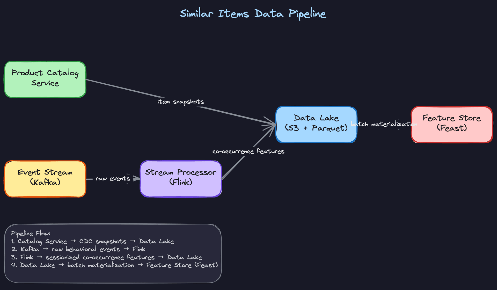
The diagram above traces the full data flow: raw Kafka events and CDC catalog snapshots land in S3, a daily Spark job processes them into clean Parquet, and the resulting co-view pairs and item feature snapshots get materialized into Feast for online serving. Each stage is partitioned by date so you can reconstruct any historical training run exactly.
Offline storage layout follows a standard lakehouse pattern. Raw Kafka events land in S3 in their original format, partitioned by date and event type. A daily Spark job processes them into Parquet files with a clean schema. Processed item features and co-view pair counts live in the data lake and get materialized into Feast for online serving.
s3://ml-data/
  raw/
    events/year=2024/month=01/day=15/   ← raw Kafka dumps
    catalog_snapshots/2024-01-15/        ← daily CDC snapshots
  processed/
    coview_pairs/cutoff=2024-01-15/      ← training pairs, versioned by cutoff
    item_features/snapshot=2024-01-15/   ← feature snapshots for training
  embeddings/
    item_vectors/model_version=v3.2/     ← output of embedding training
The cutoff and snapshot partitioning is what makes time-based reproducibility possible. When you train a model with cutoff=2024-01-15, every feature used in that training run comes from data available before that date.
Key insight: The data pipeline is where most ML system design interviews go shallow. Candidates describe the model architecture in detail but hand-wave the data. Interviewers at senior and staff level will probe exactly here: "How do you handle new items that haven't been viewed yet?" and "What happens to your training data when you change your recommendation widget?" Having concrete answers to both will separate you from the majority of candidates.
Feature Engineering
The features that power a similar items system fall into two broad camps: content signals (what an item looks like, what it's called, how it's categorized) and behavioral signals (what users do with it). Your job in the interview is to show you can design both, explain how they're computed, and keep training and serving consistent. That last part is where most candidates lose points.
Feature Categories
This is fundamentally an item-to-item retrieval problem, so there's no user profile to model. Every feature you engineer describes an item, and your goal is to produce a single dense vector per item that captures enough signal to find semantically similar neighbors.
Visual features
| Feature | Type | How it's computed |
|---|---|---|
| Image embedding | float[256] | ViT or ResNet fine-tuned with contrastive loss (SimCLR) on product images |
| Dominant color histogram | float[12] | HSV color quantization over the primary product image |
| Image quality score | float | Blur detection + resolution check; used to flag low-quality inputs |
Fine-tuning matters here. A ViT pretrained on ImageNet will cluster "red dress" with "red car" because both are red. Fine-tuning on your product catalog with supervised contrastive loss, where positives are items from the same category, fixes that.
Text features
| Feature | Type | How it's computed |
|---|---|---|
| Title + description embedding | float[384] | sentence-transformers/all-MiniLM or domain-adapted BERT |
| Category path embedding | float[64] | Learned embedding over the full taxonomy path (e.g., "Clothing > Women > Dresses > Midi") |
| Brand embedding | float[32] | Lookup table trained jointly with the model; handles ~500K unique brands |
For multilingual catalogs, swap all-MiniLM for LaBSE or mBERT. Don't try to translate everything to English first. That adds latency, introduces errors, and loses nuance in product names.
Structured features
| Feature | Type | How it's computed |
|---|---|---|
| Price bucket | int (0-9) | Log-scaled bucketing: items within the same bucket are price-comparable |
| Condition | int (enum) | New / used / refurbished, one-hot encoded |
| Listing age (days) | float | (now - created_at) / 86400, clipped at 365 |
Price bucket deserves a word. Raw price is noisy across categories. A $50 item is cheap for a laptop and expensive for a phone case. Log-scaling and bucketing within category makes price a useful similarity signal instead of a confounding one.
Behavioral features
| Feature | Type | How it's computed |
|---|---|---|
| Item2Vec embedding | float[128] | Trained on co-view sessions; items appearing in similar session contexts end up close in embedding space |
| Co-purchase count (30d) | int | Aggregated from purchase event stream, joined at training time |
| Click-through rate | float | 7-day rolling CTR from impression logs |
Behavioral embeddings capture substitutability that visual and text features miss entirely. A white ceramic mug and a stainless steel travel mug look nothing alike and share few words, but users consistently view them together. Item2Vec learns that relationship.
Key insight: Cold-start items have no behavioral signal at all. Your design needs a clean fallback: content-only embeddings for new items, behavioral embeddings for warm items, and a hybrid for everything in between. Interviewers will probe this. Have a concrete answer ready.
Feature Computation
The three-tier model (batch, near-real-time, real-time) maps directly onto how stale each feature can be before it hurts recommendation quality.
Batch features
Visual and text embeddings are the most expensive to compute and the slowest to change. A nightly Spark job reads the product catalog snapshot from S3, runs items through the encoder in batches of 512, and writes the resulting vectors back to the offline store as Parquet. From there, a materialization job pushes them into the online feature store.
# Batch embedding job (runs nightly via Airflow)
from sentence_transformers import SentenceTransformer
import pandas as pd

model = SentenceTransformer("all-MiniLM-L6-v2")

def compute_text_embeddings(df: pd.DataFrame, batch_size: int = 512):
    texts = (df["title"] + " " + df["description"]).tolist()
    embeddings = model.encode(
        texts,
        batch_size=batch_size,
        show_progress_bar=True,
        normalize_embeddings=True,   # L2-normalize for cosine similarity
    )
    df["text_embedding"] = list(embeddings)
    return df
The key constraint: at 500M items, this job needs to finish in under 12 hours to meet a nightly SLA. That means running on a GPU cluster (8xA100s) with Triton handling the encoder inference, not a CPU Spark job.
Near-real-time features
Behavioral signals like co-view counts and item popularity need to refresh on the order of hours, not days. The pipeline runs Kafka events through Flink, which sessionizes views (30-minute idle timeout), computes co-occurrence counts, and writes aggregates to the feature store every 15 minutes.
# Flink streaming job (pseudocode, PyFlink syntax)
from pyflink.datastream import StreamExecutionEnvironment
from pyflink.table import StreamTableEnvironment

env = StreamExecutionEnvironment.get_execution_environment()
t_env = StreamTableEnvironment.create(env)

# Sessionize view events with 30-minute gap
t_env.execute_sql("""
    SELECT
        session_id,
        item_id,
        COUNT(*) AS view_count,
        SESSION_START(event_time, INTERVAL '30' MINUTE) AS session_start
    FROM item_view_events
    GROUP BY
        SESSION(event_time, INTERVAL '30' MINUTE),
        session_id,
        item_id
""")
The output lands in Redis with a TTL of 24 hours. Stale co-view counts are better than missing ones; the system degrades gracefully rather than failing.
Real-time features
The only feature computed at request time is the query item's embedding, and only for new items that aren't yet in the feature store. For the 99% of requests where the item is warm, you fetch the precomputed embedding from Redis in a single key lookup.
For cold-start items, the serving layer calls the text encoder directly:
# Called at serving time for items not found in feature store
def get_query_embedding(item: dict, model: SentenceTransformer) -> list[float]:
    text = f"{item['title']} {item['description']}"
    embedding = model.encode(text, normalize_embeddings=True)
    # Write back to feature store asynchronously so next request is a cache hit
    feature_store.set_async(f"item:{item['id']}:text_emb", embedding.tolist())
    return embedding.tolist()
Write-back on first access means the second request for a new item is always fast. Don't skip this step.
Feature Store Architecture
The feature store has two sides that serve completely different access patterns, and you need both.
The online store (Redis) holds precomputed item embeddings keyed by item ID. Lookups need to complete in under 5ms to stay inside the p99 latency budget. At 500M items with a 256-dim float32 embedding, that's roughly 500GB of raw vector data. You'll shard Redis across a cluster and keep only the most-accessed items hot, falling back to DynamoDB for the long tail.
The offline store (Parquet on S3) holds the full history of features used for training. Every feature has a timestamp, so you can reconstruct exactly what the model saw during training for any given item at any point in time. This is what makes debugging training-serving skew tractable.
Common mistake: Candidates design the online store but forget the offline store entirely. Then they can't explain how they'd retrain the model without recomputing all features from scratch. The offline store is what makes incremental retraining possible.
Preventing training-serving skew is the hardest operational problem in this system. The failure mode looks like this: your batch job computes text embeddings by concatenating title and description with a newline separator. Your serving code concatenates them with a space. The embeddings are slightly different. Recall@10 drops 3% and nobody knows why for two weeks.
The fix is to share the exact same featurization code between training and serving. One Python package, one function, called from both the Spark job and the serving layer:
# shared_features/item_encoder.py
# Imported by BOTH the batch training job and the online serving layer

def build_item_text(item: dict) -> str:
    """
    Canonical text representation for an item.
    Any change here requires a full embedding recompute.
    """
    title = item.get("title", "").strip()
    description = item.get("description", "").strip()[:512]  # truncate consistently
    return f"{title} {description}"
Treat this function as an API contract. Version it. Any change triggers a full recompute of the embedding index.
Fusion Strategy
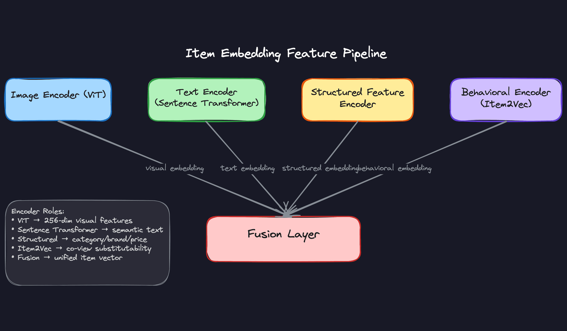
Once you have visual, text, structured, and behavioral embeddings, you need to decide how to combine them. This is a real design decision with real trade-offs, and the interviewer will likely ask you to defend your choice.
Early fusion concatenates all embeddings (or projects them through a learned fusion layer) into a single unified vector before indexing. You get one ANN index, simple serving, and a model that can learn cross-modal interactions. The downside: when behavioral embeddings are missing for cold-start items, the fused vector is incomplete and you can't easily substitute a fallback.
Late fusion maintains separate ANN indexes per modality, queries each independently, and merges the ranked lists using reciprocal rank fusion or a learned re-ranker. Cold-start is handled naturally: just skip the behavioral index for new items. The cost is higher query latency (multiple ANN calls) and a larger total index footprint.
For a catalog of 500M items with a significant cold-start population, late fusion is usually the right call. The operational complexity is worth it. That said, if your catalog is mostly warm items and you want to minimize serving latency, a hybrid approach works well: early fusion for warm items with a content-only fallback index for new ones.
Interview tip: Don't just describe these options. Tell the interviewer which one you'd pick and why, given the constraints you established in requirements. "I'd go with late fusion because we have a meaningful cold-start population and can't afford to degrade quality for new listings" is a much stronger answer than listing trade-offs and leaving it open.
Model Selection & Training
Start simple. The fastest way to lose an interviewer's confidence is to jump straight to a transformer-based hybrid model without explaining why you need it. Walk them through the progression.
Model Architecture
The Baseline
TF-IDF cosine similarity is your baseline. Vectorize item titles and descriptions, compute pairwise cosine similarity, return the top K. You can ship this in a day, it's fully interpretable, and it gives you a concrete performance floor to beat.
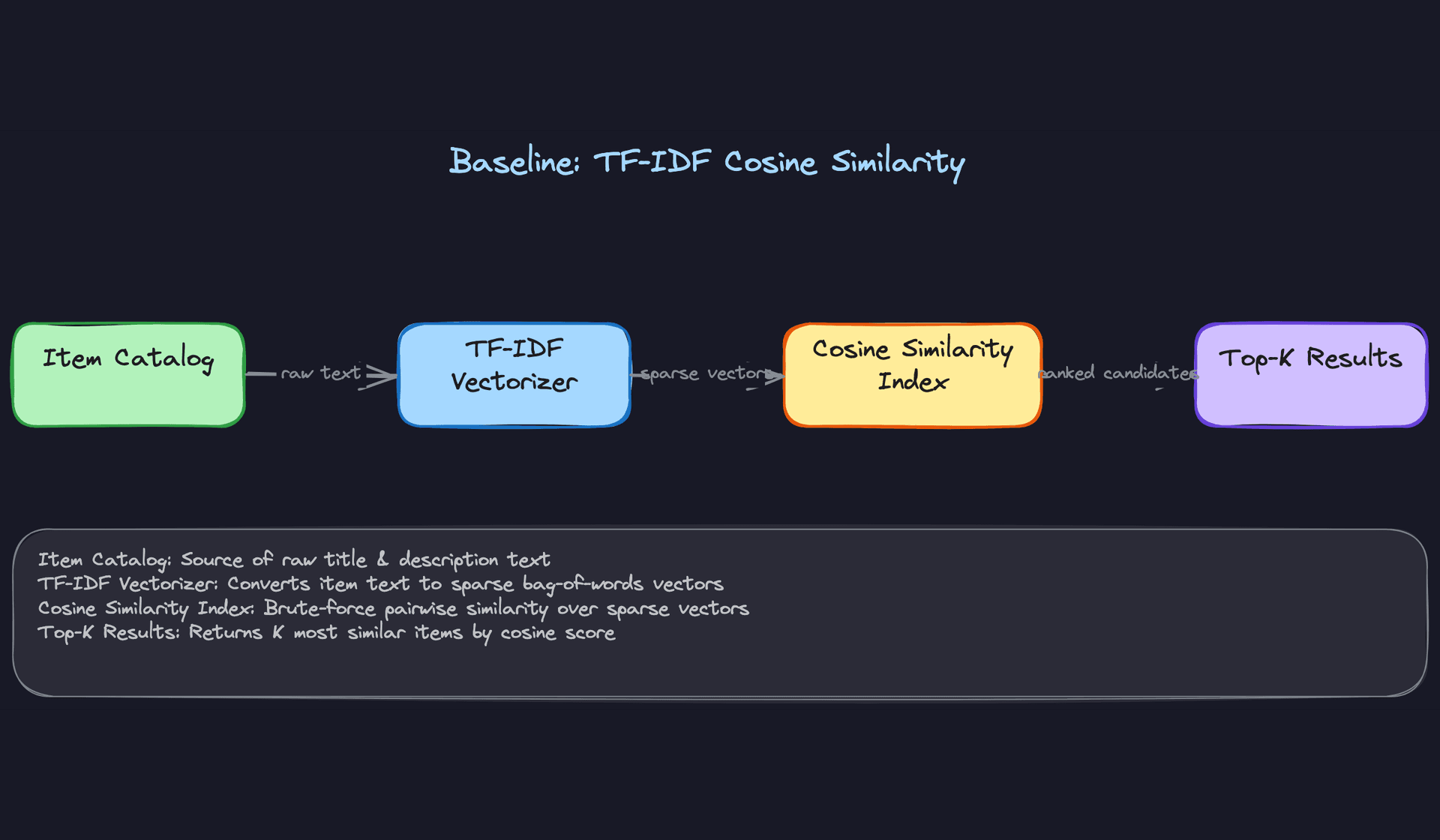
The problem is scale. Brute-force pairwise similarity over 500M items is O(n²) in memory and compute. Even at 1M items, storing a dense similarity matrix at float32 is 4TB. And TF-IDF is blind to visual similarity entirely: two identical products with different titles look unrelated.
Common mistake: Candidates propose TF-IDF as their final answer for large catalogs without acknowledging the memory and latency wall. The interviewer is waiting for you to catch this yourself.
Averaged word vectors (GloVe, fastText) are a marginal improvement. You get a dense 300-dim vector per item, which is ANN-indexable, but the embeddings aren't trained on your catalog domain and still ignore images.
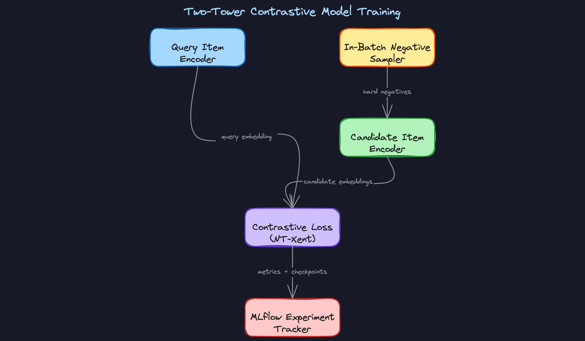
The Production Model: Content-Based Two-Tower
The right architecture for retrieval at scale is a two-tower model. One encoder for the query item, a separate encoder for candidate items. Both towers produce a fixed-size embedding, and similarity is just dot product or cosine distance in that shared space.
Why two towers instead of a cross-encoder? Because you can pre-compute and index all candidate embeddings offline. At query time, you only run the query encoder (one forward pass), then do ANN search. A cross-encoder that takes a (query, candidate) pair as joint input can't be indexed this way; you'd need to score every candidate at runtime, which is exactly the brute-force problem you're trying to avoid.
Input/output contract for the two-tower model:
# Query tower input (at inference time, single item)
{
    "item_id": str,
    "image_embedding": Tensor[256],      # from ViT encoder, frozen or fine-tuned
    "text_embedding": Tensor[128],       # from sentence transformer
    "category_id": int,
    "brand_id": int,
    "price_bucket": int                  # 0-9 quantile bucket
}

# Output: single dense vector
query_embedding: Tensor[256]            # L2-normalized, ready for ANN search

# Candidate tower produces the same shape
candidate_embedding: Tensor[256]

# Similarity score at training time
score = dot(query_embedding, candidate_embedding)  # in [-1, 1] after normalization
The loss function is temperature-scaled NT-Xent (InfoNCE). For each anchor item in a batch, the positive is an item it was co-viewed with; all other items in the batch are treated as negatives. You also mine hard negatives from behavioral logs: items that appeared in the same session but were not clicked. Hard negatives are what separate a mediocre two-tower from a good one.
def nt_xent_loss(query_emb, candidate_emb, temperature=0.07):
    # query_emb: [B, D], candidate_emb: [B, D]
    # Each row i is a positive pair; all j != i are negatives
    logits = torch.matmul(query_emb, candidate_emb.T) / temperature  # [B, B]
    labels = torch.arange(logits.size(0), device=logits.device)
    return F.cross_entropy(logits, labels)
Lower temperature sharpens the distribution and forces the model to be more discriminative. Values between 0.05 and 0.1 work well in practice; treat it as a hyperparameter you tune on validation Recall@10.
The Hybrid Model
Once the content-based two-tower is in production, you add behavioral signal. Train a third tower on co-view session data using item2vec-style skip-gram or the same contrastive objective. The behavioral tower captures substitutability: two items that users consider interchangeable even if they look different.
The fusion strategy matters here. You have two options.
Late fusion keeps separate indexes per modality and merges ranked lists at query time using reciprocal rank fusion or a learned combiner. It's operationally simpler and lets you update each modality independently.
Early fusion projects all modality embeddings through a shared linear layer into one unified vector before indexing. You get one index, lower serving complexity, but you lose the ability to update modalities independently. If your image encoder gets retrained, you rebuild the entire index.
For a 500M item catalog, early fusion with a single 256-dim unified embedding is the right call. One index is much easier to shard and serve than three. The trade-off is that retraining any modality requires a full index rebuild, which is acceptable on a weekly cadence.
class HybridItemEncoder(nn.Module):
    def __init__(self, visual_dim=256, text_dim=128, behav_dim=128, struct_dim=64, out_dim=256):
        super().__init__()
        in_dim = visual_dim + text_dim + behav_dim + struct_dim
        self.projection = nn.Sequential(
            nn.Linear(in_dim, 512),
            nn.ReLU(),
            nn.Linear(512, out_dim)
        )

    def forward(self, visual, text, behavioral, structured):
        x = torch.cat([visual, text, behavioral, structured], dim=-1)
        return F.normalize(self.projection(x), dim=-1)
Ablate each modality during evaluation. Drop behavioral embeddings and measure the Recall@10 drop. If it's small, behavioral signal isn't pulling its weight and you've added training complexity for nothing. If it's large (more than 5 points), it's earning its place.
Training Pipeline
Distributed training with PyTorch DDP across 8xA100s. The main bottleneck isn't model size (the towers are relatively small) but batch size. Contrastive learning needs large batches to get enough in-batch negatives. With 8 GPUs and a per-GPU batch size of 512, you get an effective batch of 4096, which is sufficient.
# Training config (MLflow-tracked)
training:
  gpus: 8
  per_gpu_batch_size: 512
  effective_batch_size: 4096
  learning_rate: 3e-4
  warmup_steps: 1000
  max_epochs: 20
  temperature: 0.07
  hard_negative_ratio: 0.3     # 30% of negatives are hard-mined
  checkpoint_every_n_epochs: 1
  embedding_export_path: s3://embeddings/checkpoints/
After each epoch, export the full catalog embeddings to S3. This lets you do incremental ANN index rebuilds without waiting for full training to complete. If you're running a weekly retrain, you want the index to reflect the latest checkpoint, not the model from seven days ago.
Retraining schedule: Weekly incremental retraining on a rolling 90-day behavioral window, using the previous model's weights as initialization (warm start). Monthly full retraining from scratch to prevent embedding space drift from accumulating across warm-start cycles. New items get content-only embeddings generated hourly via a lightweight batch job, separate from the main training loop.
Data windowing: 90 days of behavioral data is the sweet spot for most e-commerce catalogs. Older co-view data reflects seasonal patterns that may not generalize, and it dilutes signal from recent catalog changes. Tune this window on your validation set by comparing Recall@10 at 30, 60, 90, and 180 days.
Hyperparameter tuning with Optuna or Ray Tune over temperature, learning rate, hard negative ratio, and embedding dimension. Run 20-30 trials on a 10% data sample before committing to a full training run. The two parameters that move the needle most are temperature and hard negative ratio.
Offline Evaluation
Your primary metric is Recall@10: of the 10 items returned, what fraction are items the user actually clicked or purchased after viewing the query item? This connects directly to CTR on the widget. NDCG@10 adds position sensitivity, rewarding results that surface the best matches at rank 1 rather than rank 9.
Those two metrics alone aren't enough.
Catalog coverage measures what fraction of your 500M items ever appear in someone's Top-10 results. A model with 95% Recall@10 that only recommends from a 10K-item popularity head is useless for long-tail discovery. You want coverage above 60-70% for a healthy catalog.
Intra-list diversity catches the near-duplicate problem. If you return 10 colorway variants of the same shirt, your Recall@10 looks great but the user experience is terrible. Measure average pairwise distance within returned lists; flag any model where this drops below your threshold.
Cold-start Recall@10 is evaluated on a held-out set of items with zero behavioral history. This is a separate eval slice, not folded into the main number. A model that hits 0.45 Recall@10 overall but 0.05 on cold-start items has a serious gap you need to address before shipping.
def evaluate_model(model, test_sessions, cold_start_items, k=10):
    metrics = {}

    # Standard recall on warm items
    metrics["recall@10"] = compute_recall_at_k(model, test_sessions, k)
    metrics["ndcg@10"] = compute_ndcg_at_k(model, test_sessions, k)

    # Cold-start slice
    cold_sessions = [s for s in test_sessions if s.query_item in cold_start_items]
    metrics["cold_start_recall@10"] = compute_recall_at_k(model, cold_sessions, k)

    # Diversity
    metrics["intra_list_diversity"] = compute_avg_pairwise_distance(model, test_sessions, k)

    # Coverage
    metrics["catalog_coverage"] = compute_coverage(model, test_sessions, k)

    return metrics
Use time-based splits, not random splits. If your test set contains sessions from before your training cutoff, you're leaking future behavioral signal into training. Hold out the most recent 2 weeks of sessions as your test set, train on everything before that.
Error analysis is where most candidates skip out early. The interviewer wants to hear you think about failure modes, not just report a number.
The most common failure mode in behavioral two-towers is popularity bias. High-traffic items dominate in-batch negatives, so the model learns to push everything away from popular items rather than learning fine-grained similarity. You'll see this as a cluster of popular items that appear as "similar" to almost everything. Fix it by downsampling popular items in your negative pool.
The second failure mode is modality collapse. If your visual tower is much stronger than your text tower, the projection layer learns to ignore text entirely. Ablation metrics catch this, but you can also visualize the gradient norms per modality during training. If text gradients are near zero, you have a problem.
Tip: When the interviewer asks "how do you know the model is working?", don't just say Recall@10. Walk through cold-start performance, catalog coverage, and at least one failure mode you'd look for. That's the answer that signals senior-level thinking.
Inference & Serving
The core serving question for a similar items system isn't "how do we run the model?" It's "how do we make 500 million item embeddings queryable in under 100ms?" The model inference part is almost the easy bit.
Serving Architecture
Online vs. batch: why you need both
This system runs in a hybrid mode, and you should be able to explain why without being asked. Generating embeddings for 500M items in real-time is a non-starter at 50K QPS. Instead, you run a nightly batch job to encode the full catalog and build the ANN index offline. The online path then becomes a fast lookup: fetch the query item's precomputed embedding, run ANN search, apply filters, return results. No GPU required at query time.
The one exception is new items. A product listed an hour ago doesn't have a slot in last night's index. That's your cold-start path, and it needs a separate design (covered below).
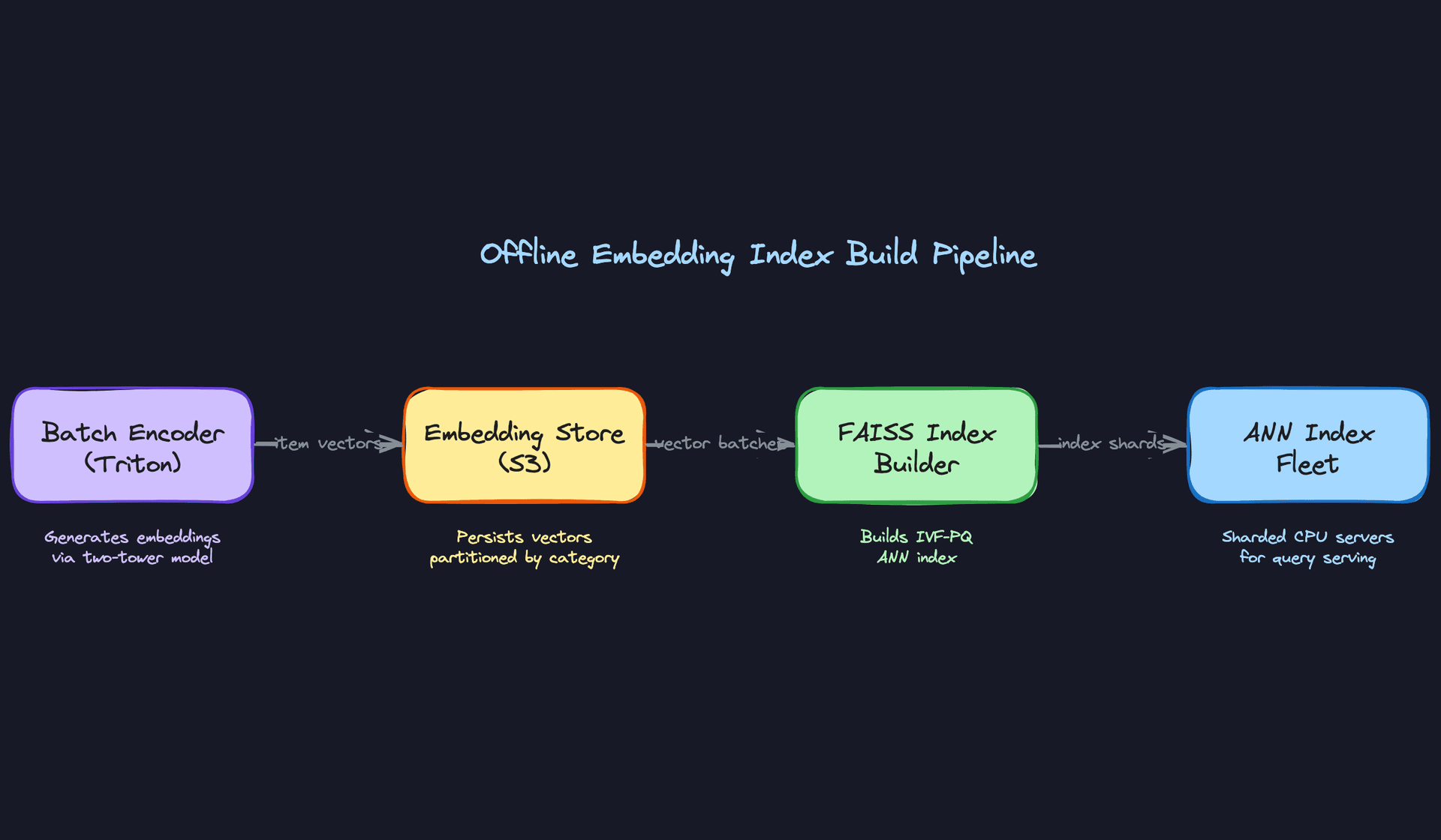
Offline index build
The batch encoder runs on Triton Inference Server backed by A100s. You're encoding 500M items, so throughput matters more than latency here. Triton's dynamic batching can saturate GPU memory efficiently, and you can partition the catalog by category to parallelize across workers.
The output is a flat file of (item_id, embedding_vector) pairs written to S3, partitioned by category. From there, FAISS index builder reads those vectors and constructs an IVF-PQ index. IVF (inverted file index) partitions the vector space into clusters so you only search a fraction of the index per query. PQ (product quantization) compresses each 256-dim float32 vector from 1KB down to roughly 64 bytes, which is what makes 500M vectors fit in memory at all.
Key insight: At 500M items with 256-dim float32 embeddings, your raw vector data is 500M × 256 × 4 bytes = 512GB. That doesn't fit on a single machine. IVF-PQ brings this down to roughly 32GB, which does. This is why quantization isn't optional at this scale.
The recall vs. latency trade-off in FAISS is controlled by nprobe, the number of IVF clusters searched per query. Higher nprobe means better recall but slower queries. You'll want to benchmark this on your actual data: a typical operating point is nprobe=64 on an index with 4096 clusters, giving ~95% recall at ~5ms per query.
Online serving path
At query time, the flow looks like this:
- API Gateway receives
GET /similar?item_id=X&k=20 - Redis cache is checked first. The top-10% of items by traffic have precomputed Top-K results cached, generated by a nightly batch job that queries the main ANN index for each high-traffic item and writes the results to Redis. TTL is aligned to your catalog update cadence (typically 6-24 hours).
- On cache miss, the item's embedding is fetched from Feast (the feature store). This is a key-value lookup by item ID, targeting sub-5ms p99
- The embedding is sent to the ANN index fleet via gRPC
- The index returns 100 candidate IDs (you over-fetch to give the post-filter room to work)
- Post-filter applies business rules: in-stock check, category constraints, diversity deduplication to remove near-identical colorways
- Top-K results returned to the caller

Latency breakdown
At p99, your budget is 100ms. Here's where it goes:
| Stage | Target p99 |
|---|---|
| Redis cache hit | ~2ms (end-to-end) |
| Feature store lookup (Feast) | ~5ms |
| ANN query (FAISS, nprobe=64) | ~10ms |
| Post-filter + ranking | ~3ms |
| Network + serialization | ~5ms |
| Total (cache miss path) | ~23ms |
That's comfortable headroom. The danger is the cold-start path, where you're recomputing the embedding on the fly. That adds GPU inference latency, which brings us to the next piece.
Cold-start path
New items fall back to a content-only embedding computed at listing time. When a seller uploads a product, a lightweight inference job runs immediately: image through the ViT encoder, title through the sentence transformer, structured features concatenated. This embedding gets written to Feast and inserted into a shadow index rebuilt every hour.
The shadow index is a small FAISS flat index (exact search, not ANN) because the new-item population is small enough that brute-force is fine. Results from the shadow index are merged with results from the main index at query time, with the post-filter handling deduplication.
Common mistake: Candidates often say "new items fall back to content embeddings" without explaining how those embeddings get into the index or how quickly. The interviewer will push on this. Have a concrete answer: embedding computed at listing time, shadow index rebuilt hourly, items appear in results within 1-2 hours of listing.
Optimization
Model optimization
The encoder model itself doesn't run at query time for warm items, so model optimization effort should be focused on the batch encoding job, not the online path. That said, faster batch encoding means you can rebuild the index more frequently, which improves freshness.
For the batch encoder, INT8 quantization via TensorRT (integrated with Triton) typically cuts encoding time by 40-50% with less than 1% recall degradation on retrieval benchmarks. Worth doing. Knowledge distillation is another option if you want to shrink the model for the cold-start real-time path: distill the full ViT into a smaller MobileViT that runs in ~10ms on CPU.
Batching
Triton's dynamic batching is your friend for the offline job. Set a max batch size of 256 and a max queue delay of 5ms. At 50K QPS of encoding requests, you'll saturate GPU throughput and see 3-4x better cost efficiency compared to single-sample inference.
For the online cold-start path, you're not batching individual user requests together (the latency budget doesn't allow it). But you can batch the embedding computation for a burst of newly listed items using a micro-batch queue with a 100ms flush interval.
GPU vs. CPU serving
The ANN index runs on CPU, not GPU. FAISS IVF-PQ search is memory-bandwidth bound, and modern CPUs with AVX-512 handle it well. GPU-accelerated FAISS exists but adds complexity and cost without meaningful latency improvement for this query pattern.
GPU is reserved for the batch encoder and the real-time cold-start encoder. Keep these concerns separate in your deployment topology.
Interview tip: If the interviewer asks why you're not using GPU for ANN search, the answer is: FAISS IVF-PQ on CPU with AVX-512 hits 5-10ms per query, which fits the budget. GPU FAISS adds operational complexity (GPU memory management, driver versions) for marginal gain at this scale. The cost-benefit doesn't pencil out unless you're running billions of vectors.
Fallback strategies
When the ANN service is degraded, you have two fallback tiers. First, serve from the Redis cache even if the TTL has expired (stale-while-revalidate). Second, if the item has no cache entry at all, fall back to a precomputed "popular items in this category" list. It's not personalized, but it's better than a blank widget. Never let the similar items slot return empty.
Online Evaluation & A/B Testing
Traffic splitting
Model experiments use item-level assignment, not user-level. An item is deterministically assigned to control or treatment based on hash(item_id) % 100 < treatment_percent. This ensures that all users viewing the same product see the same similar items, which avoids within-session inconsistency and makes the experiment cleaner to analyze.
Start at 5% traffic for a new model version. If error rates and latency look clean after 24 hours, ramp to 20%, then 50%, then full rollout. Each ramp gate requires a human sign-off or an automated check against your guardrail metrics.
Online metrics
Your primary metric is CTR on the similar items widget. Secondary metrics are add-to-cart rate from similar items clicks and session depth (did the user continue browsing after clicking a similar item?). These are your north star signals.
Track guardrail metrics in parallel: p99 latency, error rate, and null result rate (how often the widget returns fewer than K items). A model that improves CTR by 2% but increases p99 latency by 30ms is not a win.
For statistical methodology, use a two-sided t-test on CTR with a minimum detectable effect of 0.5% relative lift. At 50K QPS, you'll accumulate enough impressions for 95% power within 48-72 hours. Don't call the experiment early.
Interleaving
For ranking experiments specifically, interleaving is more statistically efficient than A/B testing. Instead of splitting traffic, you interleave results from two rankers in a single response and track which model's results get clicked. This controls for item-level variance and can detect smaller effects with less traffic. It's worth mentioning at the staff level; most candidates don't bring it up.
Key insight: The deployment pipeline is where most ML projects fail in practice. A model that can't be safely deployed and rolled back is a model that won't ship.
Deployment Pipeline
Validation gates
Before any model version touches production traffic, it must pass three gates:
- Offline recall gate: Recall@10 on the held-out eval set must be within 2% of the current production model (or better)
- Latency gate: p99 ANN query latency on a shadow load test must be under 15ms
- Diversity gate: intra-list diversity score must not regress by more than 5%, to catch embedding collapse
These checks run automatically in the CI pipeline after every training run. A model that fails any gate doesn't get promoted to the candidate registry.
Canary deployment
Promoted models go through a canary phase before full rollout. The canary receives 1% of live traffic for 6 hours. During this window, you're watching for latency regressions, error rate spikes, and any anomalies in the embedding distribution (a sudden shift in average cosine similarity of returned results is a red flag).
If the canary is clean, automated ramp-up proceeds: 5% → 20% → 50% → 100%, with a 12-hour hold at each stage.
Shadow scoring
Before the canary phase, run the new model in shadow mode: it scores every request alongside the production model but its results are discarded. This lets you compare embedding distributions and result overlap between old and new models on real traffic without any user-facing risk. If shadow results diverge significantly from production (less than 60% overlap in Top-10), that's a signal to investigate before proceeding.
Rollback triggers
Rollback is automatic if any of the following are breached during rollout:
- p99 latency exceeds 50ms for more than 5 minutes
- Error rate on the similarity service exceeds 0.5%
- CTR on the similar items widget drops more than 10% relative to the control group
Rollback means flipping the traffic split back to the previous model version. Because embeddings are versioned in S3 and the FAISS index build is reproducible, you can also roll back the index itself if the issue is in the vectors rather than the serving code.
# Simplified rollback trigger in Airflow
def check_rollback_conditions(model_version: str, window_minutes: int = 5):
    metrics = fetch_metrics(model_version, window_minutes)

    if metrics["p99_latency_ms"] > 50:
        trigger_rollback(model_version, reason="latency_breach")
    elif metrics["error_rate"] > 0.005:
        trigger_rollback(model_version, reason="error_rate_breach")
    elif metrics["ctr_relative_change"] < -0.10:
        trigger_rollback(model_version, reason="ctr_regression")
Interview tip: When you describe your deployment pipeline, the interviewer wants to hear that you've thought about failure modes, not just the happy path. Mention shadow scoring and automatic rollback triggers unprompted. It signals you've shipped models before, not just trained them.
Monitoring & Iteration
Most candidates design a great launch-day system and stop there. The interviewer is watching to see if you understand that a similarity system degrades silently. No crashes, no 500s, just quietly worse recommendations as the catalog shifts and user behavior evolves.
Tip: Staff-level candidates distinguish themselves by discussing how the system improves over time, not just how it works at launch.
Production Monitoring
Input distribution drift is your first line of defense. Track the distribution of incoming item embeddings using summary statistics (mean cosine norm, per-dimension variance) and flag when they diverge from the training distribution. A sudden spike in missing images or truncated descriptions upstream will corrupt embeddings before any model metric catches it.
For schema violations, instrument your feature ingestion pipeline to count null rates per feature column daily. If the category_id field starts arriving as a string instead of an integer because some upstream team changed their schema, your structured encoder silently produces garbage. You want an alert before that reaches the index.
Model monitoring on a retrieval system is trickier than classification because you don't have a ground-truth label per query. Instead, track the distribution of the similarity scores returned by the ANN index. Plot the p10, p50, and p90 cosine similarity of Top-K results over time. A downward drift in p50 similarity means the index is returning less relevant results, whether from embedding drift, a bad model push, or index corruption.
You can also monitor prediction distribution shift indirectly through diversity metrics. If intra-list diversity suddenly collapses (all 10 results are nearly identical), that's a signal of embedding collapse in a recent training run. If diversity explodes (results look random), the index may have been rebuilt with stale or mismatched embeddings.
System monitoring is table stakes but easy to get wrong at this scale. At 50K QPS with 500M vectors sharded across a CPU fleet, you need per-shard latency histograms, not just aggregate p99. A single hot shard serving popular items can blow your SLA while the aggregate looks fine. Track ANN query latency, feature store lookup latency, and post-filter latency separately so you can isolate bottlenecks.
For index freshness, instrument the pipeline to record the timestamp when each item's embedding first appears in ANN query results. Compare that to the item's created_at timestamp in the catalog. If the median lag exceeds your 2-hour SLA, alert immediately. This is the metric most teams forget to build until a seller complains their new listing isn't showing up anywhere.
Alerting thresholds should be tiered. P0: ANN service error rate above 1%, or feature store p99 latency above 50ms. P1: embedding drift score (MMD against training distribution) above threshold, or index freshness lag above SLA. P2: business metric regression (CTR down more than 5% week-over-week) that persists for more than 24 hours. Don't page someone at 2am for a CTR blip.
Feedback Loops
Every click, add-to-cart, and purchase on the similar items widget is a training signal. The pipeline for capturing it looks like this: the frontend logs an impression event with the query item ID, the ranked result IDs, and the position. A click or conversion event joins back to that impression. Flink sessionizes and deduplicates these within a 30-minute window, then writes co-interaction pairs to the data lake for the next training run.
Feedback delay is the real problem. A user clicks a similar item today but converts three days later after comparison shopping. If you train on clicks only, you're optimizing for curiosity, not purchase intent. The standard approach is to use a delayed label window: hold back training examples for 72 hours before finalizing their label, so late conversions can join. This means your training data is always slightly stale, which is a deliberate trade-off.
For items with very low traffic (long-tail catalog), you may wait weeks for enough behavioral signal to be useful. In that window, the item relies entirely on content embeddings. Design your pipeline to track per-item behavioral signal count and automatically graduate items from the content-only index to the hybrid index once they cross a minimum interaction threshold (say, 50 co-views).
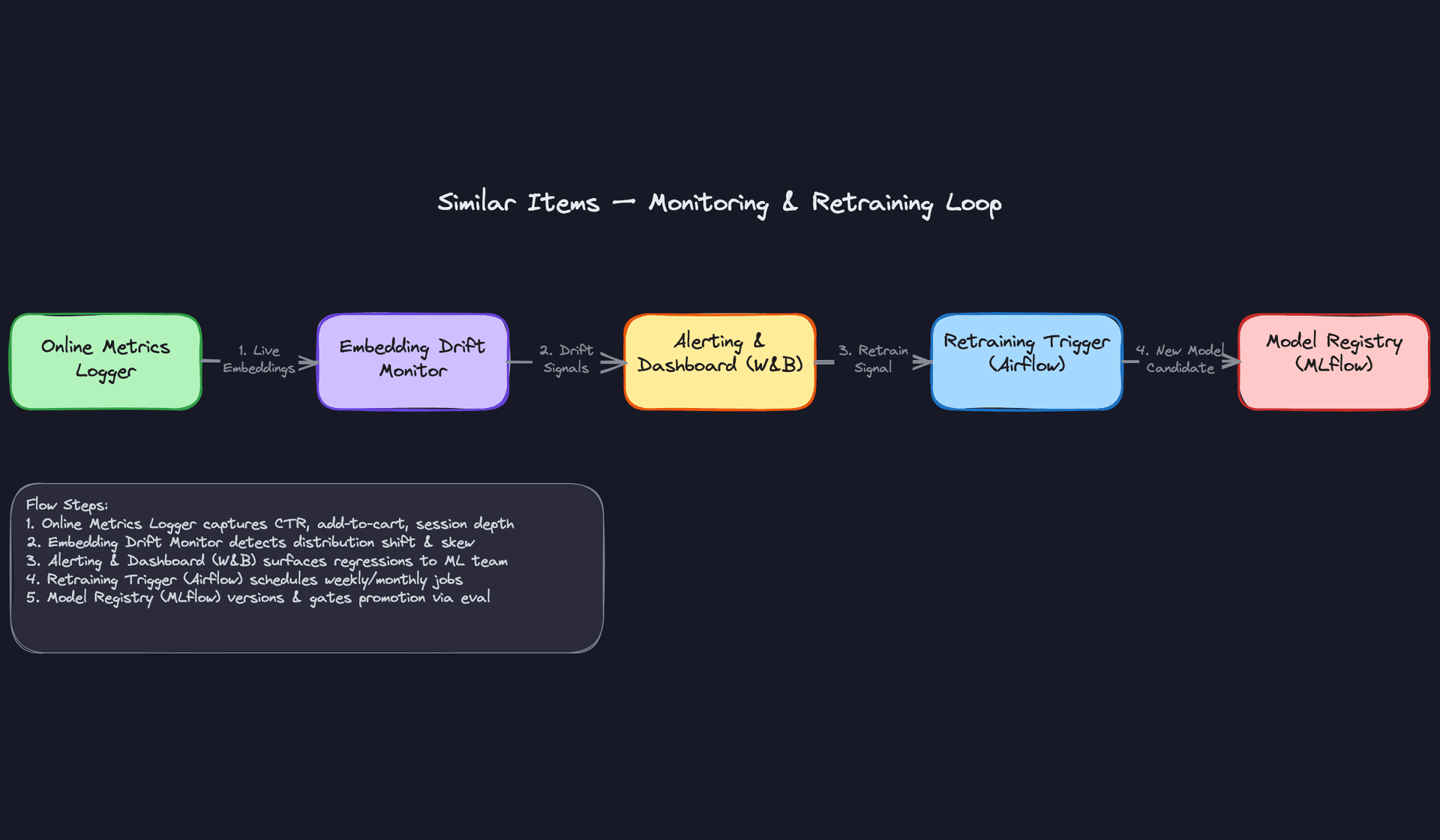
Closing the loop from alert to redeployment should be a defined runbook, not an ad-hoc process. An embedding drift alert triggers a diagnosis checklist: check feature pipeline health first (is the data bad?), then check the index build logs (did a rebuild fail silently?), then compare the live embedding distribution to the last known-good checkpoint. If the data pipeline is healthy and the index is fresh, that's your signal to trigger retraining. The retraining job promotes a new model candidate to the registry, which gates on offline Recall@10 before any traffic is shifted.
Continuous Improvement
Retraining strategy is a question of cost versus freshness. Weekly incremental retraining on fresh behavioral data using the previous model as a warm start is cheap and keeps behavioral embeddings current. Monthly full retraining from scratch prevents the embedding space from drifting too far from the original geometry, which happens when warm-start updates compound over many cycles. Think of it like git: incremental commits are fast, but you occasionally need a clean branch.
Drift-triggered retraining is worth building once you have stable monitoring. When MMD between live and training embeddings crosses a threshold, or when CTR drops and holds for 48 hours, automatically kick off an incremental retrain. This is more responsive than a fixed schedule and avoids wasting compute on weeks when nothing has changed.
Prioritizing model improvements is where staff-level thinking shows. Early in the system's life, data quality fixes (better image preprocessing, deduplicating near-identical listings) will outperform any architecture change. Once data quality is high, adding modalities (video thumbnails, review text) tends to help more than tuning hyperparameters. Architecture changes (switching from item2vec to a transformer-based behavioral encoder) are expensive to validate and should be reserved for when you have clear evidence the current architecture is the bottleneck, not the data.
As the system matures, the interesting problems shift. At launch, cold-start is your biggest gap. After six months, popularity bias in behavioral embeddings becomes the dominant failure mode: the model learns that everything is similar to bestsellers because they appear in every co-view session. Correcting for this requires explicit popularity debiasing during training, or a diversity-aware re-ranking layer that penalizes results dominated by a few high-traffic items.
Key insight: A mature similar items system is less about the model and more about the feedback infrastructure. The team that wins long-term is the one that can run clean A/B tests, iterate on data quality, and detect regressions before users notice them.
Long-term, the architecture itself evolves. You start with a single unified index. As the catalog grows and diversifies (fashion vs. electronics vs. groceries), you'll find that per-category specialized models outperform a single global model because the notion of "similar" is fundamentally different across domains. The monitoring system you build now needs to support per-category metric tracking from day one, even if you start with a single model, so you can identify which categories are underserved and prioritize accordingly.
What is Expected at Each Level
Interviewers calibrate their expectations based on your level, but one thing is true across the board: vague answers get you nowhere. "We'd use embeddings and find similar items" is not a design. Here's what actually separates the levels.
Mid-Level
- Frames the problem correctly as a retrieval task, not a ranking task. Knows that brute-force similarity over 500M items is a non-starter and reaches for ANN search without being prompted.
- Proposes a reasonable embedding strategy. Content-based (visual + text) is a solid starting point. You don't need to design the full hybrid pipeline, but you should be able to justify your choice.
- Sketches a working serving path: item ID in, embedding lookup, ANN query, Top-K out. Mentions caching for high-traffic items.
- Defines at least one offline evaluation metric. Recall@10 is the obvious one. Bonus points for mentioning catalog coverage or intra-list diversity.
Common mistake: Mid-level candidates often describe the ML model in detail but leave the serving path as a hand-wave. "Then we deploy it" is not a system design answer.
Senior
- Handles cold-start concretely. Not just "new items fall back to content embeddings" but explaining how: a shadow index rebuilt hourly, separate from the main behavioral index, with a promotion path once behavioral signal accumulates.
- Reasons about index freshness as an SLA. Knows that a nightly batch rebuild is fine for warm items but unacceptable for a marketplace where new listings need to appear in recommendations within hours.
- Discusses FAISS quantization trade-offs. IVF-PQ compresses aggressively and fits more vectors in memory; HNSW gives better recall at the cost of higher memory footprint. A senior candidate picks one and explains why given the catalog size.
- Proposes a real A/B testing strategy for model rollout: holdout traffic, the specific business metrics being tracked (CTR, add-to-cart from the widget), and a minimum detectable effect size. Not just "we'd run an A/B test."
Key insight: The jump from mid to senior isn't knowing more ML. It's thinking about the system around the model: freshness, scale, and how you know the new model is actually better in production.
Staff+
- Drives toward the hard scale constraints without being asked. At 500M items, a single FAISS index doesn't fit on one machine. A staff candidate talks about index sharding, consistent hashing across the ANN fleet, and what happens during an index rebuild when traffic is live.
- Brings up training-serving skew unprompted. Periodically sampling live query embeddings and comparing their distribution to training embeddings (MMD or KL divergence) is the kind of operational detail that signals you've actually run one of these systems.
- Thinks in feedback loops. Behavioral data improves embeddings, but popularity bias in co-view data will make your recommendations collapse toward bestsellers over time. A staff candidate names this failure mode and proposes a mitigation (e.g., popularity-debiased sampling during training).
- Identifies cross-team dependencies and their failure modes. The catalog team owns item metadata freshness. The data platform team owns the feature store SLA. If either degrades, your similarity results silently get worse. Staff candidates design for that, with alerting on index freshness lag and embedding distribution shifts.
Warning: Staff-level candidates sometimes over-index on theoretical ML sophistication (custom loss functions, exotic architectures) while underspecifying the operational story. Interviewers at this level want to see system judgment, not just ML depth.
The single strongest signal across all levels is how you handle cold-start. Any candidate can acknowledge it exists. The ones who get offers explain exactly what the fallback path looks like, how long a new item stays in the cold-start regime, and what triggers the transition to the behavioral index. If you can answer that cleanly and unprompted, you're ahead of most of the field.
The red flag that tanks candidates at every level: proposing brute-force cosine similarity over the full catalog without acknowledging what that costs. At 500M items with 256-dim float32 vectors, that's 512GB just to store the vectors, and a single query becomes a matrix multiply over half a billion rows. Saying "we'd just compute cosine similarity" tells the interviewer you haven't thought about scale at all.
Key takeaway: This system lives or dies on the gap between retrieval and ranking. Retrieval (ANN search over embeddings) needs to be fast and approximate. Ranking (post-filtering, diversity, business rules) is where you apply precision. Conflating the two, or skipping the distinction entirely, is the most common mistake in similar items interviews.
