Understanding the Problem
Product definition: A search and indexing pipeline ingests documents from upstream sources, transforms and enriches them, and makes them queryable through a search index with defined freshness guarantees.
What is a Search & Indexing Pipeline?
Most applications treat search as a product feature. Data engineers treat it as a pipeline problem. Your job isn't to build the search box; it's to make sure the right documents get into the index, in the right shape, at the right time, so that the search box actually works.
The system has two distinct halves. The write path takes raw documents from a source (a database, a data lake, a CDC stream), transforms them into a queryable representation, and loads them into a search index like Elasticsearch or OpenSearch. The read path serves queries against that index. These halves have very different scaling properties and failure modes, and a good candidate keeps them clearly separated throughout the interview.
Functional Requirements
Before writing a single component, you need to pin down what kind of search you're building. Full-text search over user-generated content (product listings, articles, support tickets) looks completely different from faceted search over an analytical dataset. One needs tokenization and relevance scoring; the other needs filter-heavy queries and aggregations. Ask explicitly.
Core Requirements
- Ingest documents from a source system (database export or CDC stream) and write them to a search index
- Support full-text keyword search with relevance ranking (BM25 as the baseline)
- Reflect document updates and deletes in the index within a defined freshness window (near-real-time, targeting under 5 minutes)
- Handle bulk initial loads (full index builds) without taking the search index offline
- Track pipeline state so restarts don't produce duplicate or missing index entries
Below the line (out of scope)
- Vector similarity search and hybrid ranking (acknowledged; would require a separate embedding pipeline and a vector-capable store like Weaviate or Pinecone)
- User-facing search UI, query suggestion, and spell correction
- Multi-tenant index isolation across different business units
Note: "Below the line" features are acknowledged but won't be designed in this lesson.
Non-Functional Requirements
The numbers here shape every architectural decision downstream, so push the interviewer for specifics before you start drawing boxes.
- Scale: 1 billion documents in the index at steady state; approximately 500 million source records updated per day across all document types
- Query volume: 10,000 search QPS at peak, with p99 query latency under 200ms
- Index freshness: Updates must appear in search results within 5 minutes of the source mutation (near-real-time SLA); full index rebuilds must complete within 4 hours
- Durability: No document loss during pipeline restarts or rebalances; exactly-once indexing semantics required
- Availability: Query serving targets 99.9% uptime; the indexing pipeline can tolerate brief pauses but must self-recover without manual intervention
Back-of-Envelope Estimation
Assume 1 billion documents, each averaging 2 KB of raw content. After tokenization and enrichment, the indexed representation grows to roughly 5 KB per document (stored fields, inverted index overhead, and metadata).
| Metric | Calculation | Result |
|---|---|---|
| Total index storage | 1B docs × 5 KB | ~5 TB |
| Daily update volume | 500M updates/day ÷ 86,400s | ~5,800 updates/sec (peak ~3x = 17K/sec) |
| Streaming ingest throughput | 17K events/sec × 2 KB avg payload | ~34 MB/sec into Kafka |
| Query throughput | 10,000 QPS × ~5 KB response | ~50 MB/sec read from index |
| Bulk load bandwidth | 1B docs × 2 KB ÷ 4 hours | ~140 MB/sec from object storage |
The storage number tells you Elasticsearch will need multiple shards and replicas, probably 20+ primary shards to keep each shard under 50 GB. The 17K updates/sec peak is the number that forces you toward a streaming path rather than hourly batch jobs. Keep both in your head when you get to the design.
Tip: Always clarify requirements before jumping into design. Candidates who ask about write patterns (append-heavy vs. high-churn) and freshness SLAs before touching the architecture signal seniority immediately. The interviewer is watching for this.
The Set Up
Before sketching any pipelines, you need to be precise about what objects actually flow through this system. Candidates who blur the line between a raw source record and an indexed document end up with muddled designs that break under schema changes or pipeline restarts.
Core Entities
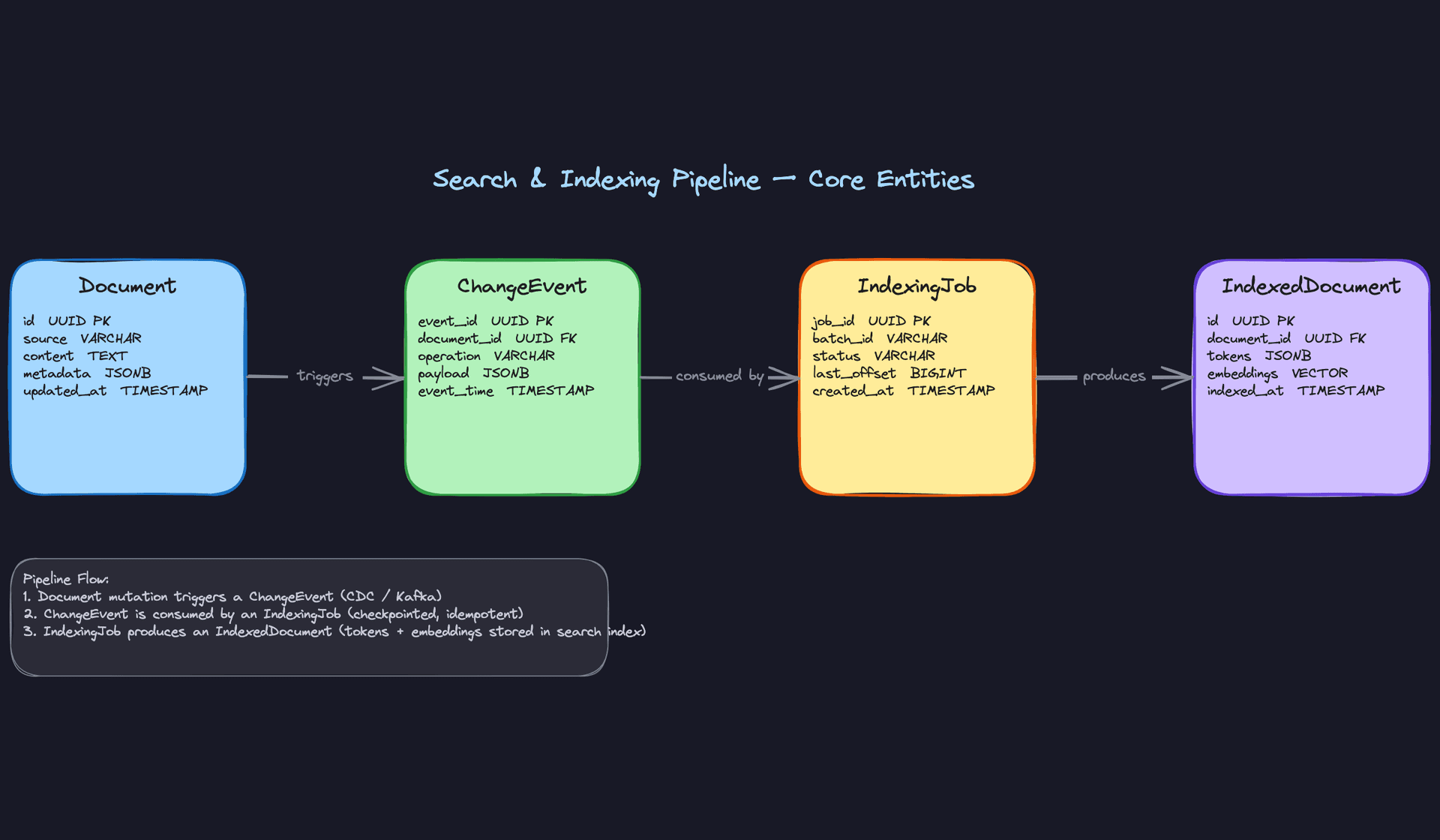
Four entities carry the weight of this design. Get comfortable explaining each one and why it exists separately.
Document is the raw source record. It comes from your upstream system, whether that's a product catalog database, a content management platform, or a log store. You don't control its shape upstream. What you do control is how you canonicalize it after ingestion into your pipeline's internal store. The schema below represents that internal canonical form, not the upstream source table itself.
ChangeEvent is the signal that something happened to a Document. In a live pipeline, these originate from streaming sources: a Debezium CDC topic, a Kafka event, a Kinesis record. The schema below is not the active streaming source. Think of it as an archive table or a replay buffer, useful for backfills, dead-letter processing, and auditing. The real-time path reads directly from the Kafka topic. All three operations (create, update, delete) need to be handled correctly, and forgetting deletes is one of the most common gaps interviewers probe for.
IndexedDocument is not just a copy of the Document with some extra fields. It's a fundamentally different object: tokenized, normalized, enriched, and shaped for query performance. The transformation between Document and IndexedDocument is where most of the pipeline complexity lives. Field extraction, NLP tokenization, embedding generation, and null handling all happen in that gap. In production, this data lives inside a specialized search engine like Elasticsearch, OpenSearch, or Solr, not in a relational table. The SQL schema below is a conceptual representation of the fields your pipeline produces and writes into that engine.
IndexingJob is the operational record for a pipeline run. It stores the last committed Kafka offset, a batch ID, and a status. Without it, a job restart has no idea where to resume, and you end up with either duplicate index entries or silent gaps.
Key insight: IndexingJob is what makes your pipeline idempotent. If a Flink job crashes mid-batch and restarts, it reads the last committed offset from IndexingJob and replays from there. The upsert into the search index is keyed on document_id, so replaying the same event twice produces the same result.-- Internal canonical store for ingested documents.
-- This is NOT the upstream source table; it's your pipeline's normalized copy.
CREATE TABLE documents (
id UUID PRIMARY KEY DEFAULT gen_random_uuid(),
source VARCHAR(100) NOT NULL, -- e.g. 'product_catalog', 'articles_cms'
content TEXT NOT NULL, -- raw text body to be indexed
metadata JSONB NOT NULL DEFAULT '{}', -- arbitrary source-specific fields
updated_at TIMESTAMP NOT NULL DEFAULT now()
);
CREATE INDEX idx_documents_updated ON documents(updated_at DESC);
-- Archive/replay table for change events. The live pipeline consumes
-- these from Kafka directly; this table serves backfills, audits, and dead-letter replay.
CREATE TABLE change_events (
    event_id     UUID PRIMARY KEY DEFAULT gen_random_uuid(),
    document_id  UUID NOT NULL REFERENCES documents(id),
    operation    VARCHAR(10) NOT NULL,            -- 'CREATE', 'UPDATE', 'DELETE'
    payload      JSONB NOT NULL DEFAULT '{}',     -- full or partial document snapshot
    event_time   TIMESTAMP NOT NULL DEFAULT now()
);

CREATE INDEX idx_change_events_document ON change_events(document_id, event_time DESC);
-- Conceptual schema for what the pipeline writes into the search engine
-- (e.g. Elasticsearch, OpenSearch). In practice, this lives as an index mapping
-- in your search engine, not as a relational table. The VECTOR type here is
-- illustrative; production vector search uses dedicated engines like Pinecone or
-- the kNN capabilities built into OpenSearch/Elasticsearch.
CREATE TABLE indexed_documents (
    id             UUID PRIMARY KEY DEFAULT gen_random_uuid(),
    document_id    UUID NOT NULL REFERENCES documents(id),
    tokens         JSONB NOT NULL DEFAULT '{}',     -- extracted and normalized token map
    embeddings     VECTOR(1536),                    -- dense vector for similarity search; nullable until enrichment completes
    schema_version INT NOT NULL DEFAULT 1,          -- tracks which index template version produced this record
    indexed_at     TIMESTAMP NOT NULL DEFAULT now()
);

CREATE UNIQUE INDEX idx_indexed_documents_doc ON indexed_documents(document_id);
The schema_version column is not decoration. When you evolve your index mapping, you need to know which documents were built under the old template so you can backfill them selectively. In Elasticsearch terms, this maps to an index alias strategy where you build a new index under a versioned name and cut the alias over when the backfill completes.
CREATE TABLE indexing_jobs (
    job_id       UUID PRIMARY KEY DEFAULT gen_random_uuid(),
    batch_id     VARCHAR(255) NOT NULL UNIQUE,    -- idempotency key; safe to retry with same batch_id
    status       VARCHAR(20) NOT NULL DEFAULT 'RUNNING',  -- 'RUNNING', 'COMPLETE', 'FAILED'
    last_offset  BIGINT NOT NULL DEFAULT 0,       -- last committed Kafka offset per partition group
    error_msg    TEXT,                            -- populated on failure for debugging
    created_at   TIMESTAMP NOT NULL DEFAULT now(),
    updated_at   TIMESTAMP NOT NULL DEFAULT now()
);

CREATE INDEX idx_indexing_jobs_status ON indexing_jobs(status, created_at DESC);
API Design
The API surface here is deliberately thin. The indexing pipeline is mostly internal infrastructure, so the external-facing endpoints are limited to query serving and pipeline management. Don't over-design this layer; interviewers want to see you focus on the data path, not REST conventions.
// Submit a search query and return ranked results
GET /search?q={query}&page={page}&limit={limit}&source={source}
-> {
     "results": [
       { "document_id": "uuid", "score": 0.94, "snippet": "...", "metadata": {} }
     ],
     "total": 1042,
     "page": 1,
     "latency_ms": 18
   }
// Trigger a full or partial index rebuild job
POST /indexing/jobs
{
  "batch_id": "rebuild-2024-06-01",
  "source": "product_catalog",
  "mode": "full" | "incremental",
  "since": "2024-05-31T00:00:00Z"   // only used when mode = "incremental"
}
-> {
     "job_id": "uuid",
     "status": "RUNNING",
     "created_at": "2024-06-01T02:00:00Z"
   }
// Check the status of an indexing job (used by orchestration and monitoring)
GET /indexing/jobs/{job_id}
-> {
     "job_id": "uuid",
     "batch_id": "rebuild-2024-06-01",
     "status": "COMPLETE",
     "last_offset": 8842901,
     "updated_at": "2024-06-01T03:14:22Z"
   }
// Ingest a single document or a small batch (used by low-volume upstream systems without CDC)
POST /documents
{
  "source": "articles_cms",
  "documents": [
    { "id": "uuid", "content": "...", "metadata": { "author": "...", "tags": [] } }
  ]
}
-> {
     "accepted": 1,
     "rejected": 0
   }
GET /search uses a GET verb because it's a read with no side effects, and query parameters are appropriate for filter facets. The POST /indexing/jobs endpoint uses POST because triggering a rebuild creates a new job resource. POST /documents follows the same logic for document ingestion.
Common mistake: Candidates sometimes design a PUT /documents/{id} endpoint for updates and wire it directly to the search index. Don't do this. Document mutations should flow through the change event pipeline, not bypass it. Direct writes to the index skip your enrichment step and break idempotency tracking.One thing worth flagging for the interviewer: in most production setups, /search is the only endpoint that external clients ever touch. The indexing and document ingestion endpoints are internal, often called only by Airflow DAGs or CI/CD pipelines. Framing it that way shows you understand the operational boundary.
High-Level Design
Start by splitting the problem into three concerns: getting documents into the index, keeping them fresh as they change, and serving queries against them. Most candidates jump straight to Elasticsearch and handwave the pipeline. The interviewer wants to see you think about data movement, not just storage.
1) Batch Indexing Path
The batch path is your foundation. It handles the initial full load and periodic full rebuilds, and it's where you'll process the bulk of your document corpus.
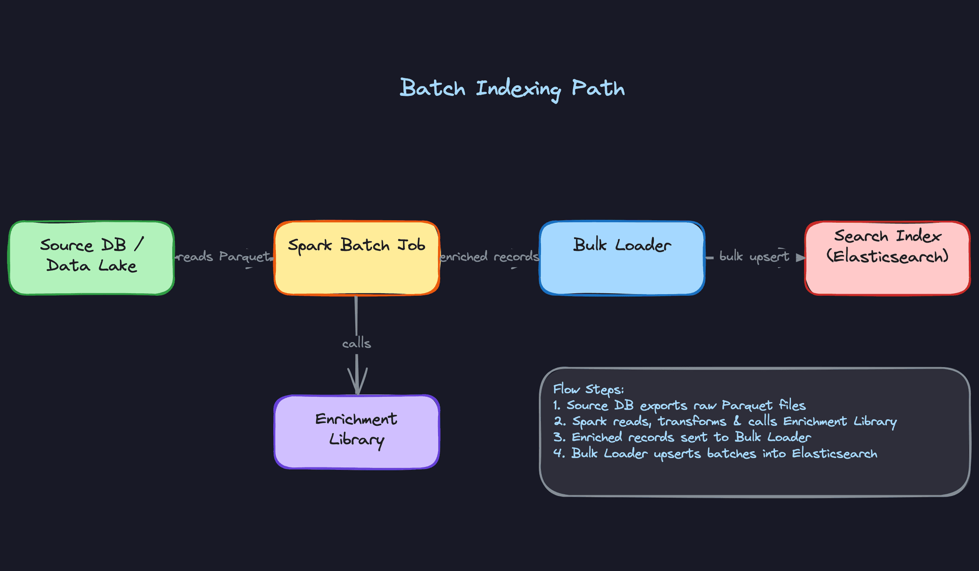
Core components: - Source data lake (S3 or GCS) storing raw documents as Parquet - Spark batch job for reading, transforming, and enriching documents - Enrichment library (shared, more on this below) - Bulk loader to push enriched records into Elasticsearch - Elasticsearch or OpenSearch as the search index
Data flow:
- Raw documents land in S3, partitioned by source and date (e.g.,
s3://data-lake/documents/source=catalog/date=2024-01-15/). - An Airflow DAG triggers the Spark job on a schedule, passing the target partition range.
- Spark reads the Parquet files, applies field extraction and normalization via the enrichment library, and produces enriched records.
- Enriched records are written back to a staging Parquet location for auditability, then passed to the bulk loader.
- The bulk loader calls the Elasticsearch Bulk API in batches of 1,000 to 5,000 documents, using
_idset to the document's UUID for idempotent upserts. - The Airflow DAG marks the run complete and updates the
IndexingJobcheckpoint table.
# Spark batch enrichment job (simplified)
from pyspark.sql import SparkSession
from enrichment_lib import normalize_fields, extract_tokens

spark = SparkSession.builder.appName("batch-indexer").getOrCreate()

docs = spark.read.parquet("s3://data-lake/documents/date=2024-01-15/")

enriched = (
    docs
    .withColumn("tokens", extract_tokens("content"))
    .withColumn("normalized_title", normalize_fields("title"))
    .withColumn("indexed_at", current_timestamp())
    .select("id", "source", "tokens", "normalized_title", "metadata", "indexed_at")
)

# Write staging copy for auditability
enriched.write.mode("overwrite").parquet("s3://data-lake/indexed/date=2024-01-15/")

# Bulk load into Elasticsearch
enriched.foreachPartition(bulk_upsert_to_es)
The key design decision here is using the document UUID as the Elasticsearch _id. This makes every write idempotent: if the Spark job fails halfway and restarts, re-indexing the same documents won't create duplicates. Don't use Elasticsearch's auto-generated IDs for a pipeline you control.
Common mistake: Candidates often propose writing directly from Spark to Elasticsearch without a bulk loader abstraction. Elasticsearch has back-pressure limits. You need retry logic, batch sizing, and circuit breaking. The bulk loader handles all of that in one place.
The trade-off with batch is freshness. If you run nightly, documents updated at 9 AM won't appear in search until the next morning. That's fine for some use cases (archival search, analytics catalogs) and completely unacceptable for others (product inventory, news articles). That's what the streaming path solves.
2) Streaming Indexing Path
The streaming path handles incremental updates: new documents, edits, and deletes that need to appear in search within seconds or minutes rather than hours.
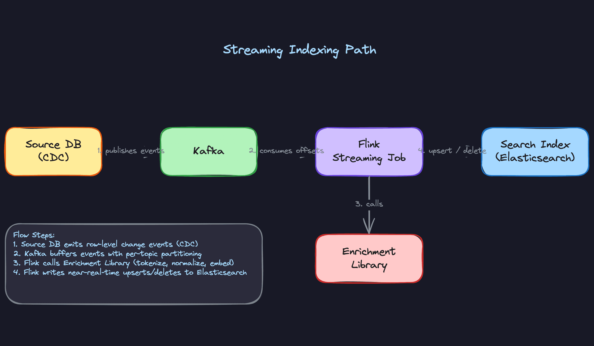
Core components: - Source database with CDC enabled (Debezium reading from Postgres WAL, for example) - Kafka as the durable change event bus - Flink streaming job consuming and processing events - Same enrichment library used by the batch path - Elasticsearch receiving near-real-time upserts and deletes
Data flow:
- A row changes in the source database. Debezium captures the WAL entry and publishes a
ChangeEventto a Kafka topic (e.g.,documents.changes), partitioned bydocument_id. - The Flink job consumes from that topic, maintaining per-partition offsets in its checkpoint state.
- For each event, Flink calls the enrichment library to tokenize and normalize the document payload.
- Flink writes to Elasticsearch using the operation type from the event:
indexfor creates and updates,deletefor deletes. - Flink checkpoints its Kafka offsets to S3 every 30 seconds (configurable). On restart, it resumes from the last committed checkpoint, not from the beginning of the topic.
# Flink Kafka consumer config (PyFlink, simplified)
kafka_source = KafkaSource.builder() \
    .set_bootstrap_servers("kafka:9092") \
    .set_topics("documents.changes") \
    .set_group_id("search-indexer") \
    .set_starting_offsets(OffsetsInitializer.committed_offsets()) \
    .set_value_only_deserializer(ChangeEventDeserializer()) \
    .build()

env.from_source(kafka_source, WatermarkStrategy.no_watermarks(), "Kafka Source") \
   .map(enrich_document) \
   .add_sink(ElasticsearchSink(es_client, index_name="documents"))
Partitioning Kafka by document_id is deliberate. It guarantees that all events for a given document are processed in order by the same Flink task. Without this, an update could be processed before the create, leaving the document in a corrupt state.
Interview tip: When the interviewer asks "what happens if Flink restarts mid-batch?", your answer is: Flink replays from the last checkpoint. Because Elasticsearch upserts are idempotent (keyed on document ID), replaying events produces the same result. This is at-least-once delivery with idempotent writes, which is effectively exactly-once from the index's perspective.
The streaming path adds operational complexity. You now have two pipelines to monitor, two failure modes to handle, and two places where enrichment logic could diverge. That last point is why the enrichment library matters so much.
3) Query Serving Layer
The query layer is intentionally thin. Its job is to translate, not to compute.
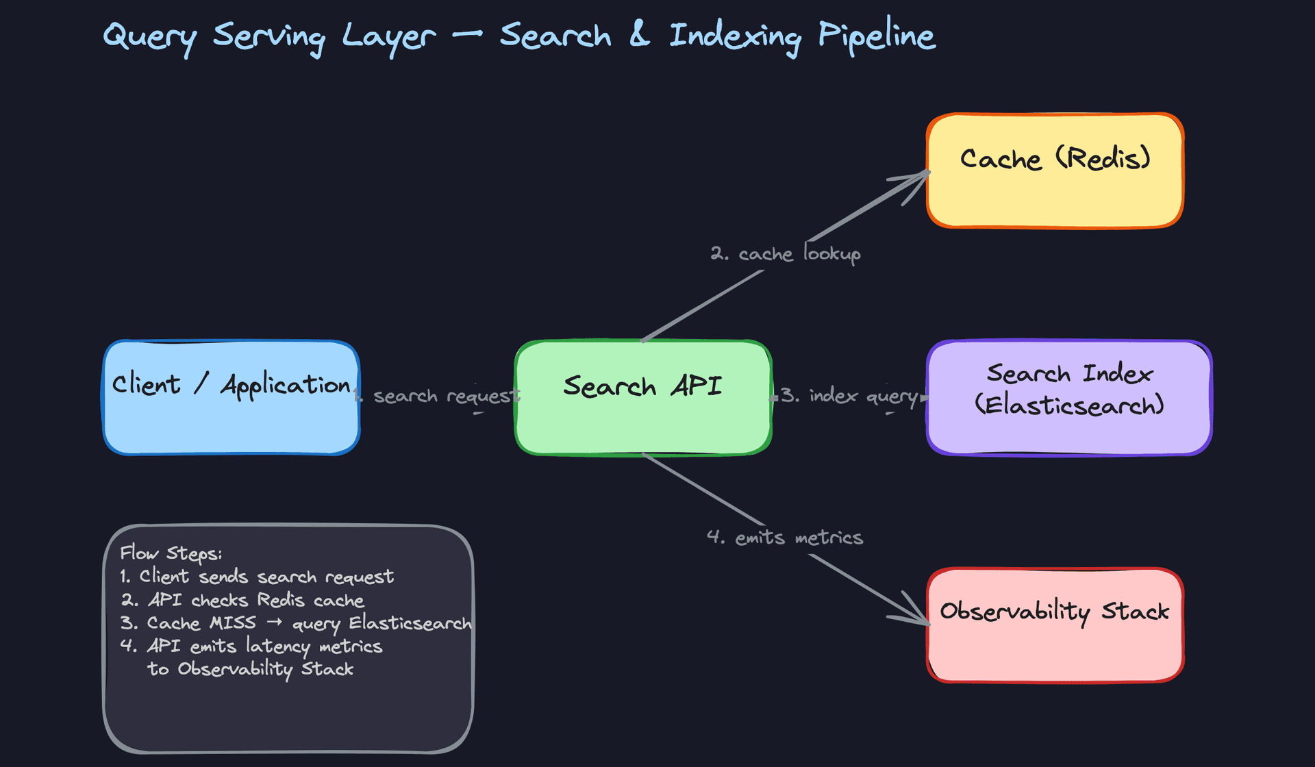
Core components: - Client application issuing search requests - Search API (stateless REST service) - Redis cache for frequent queries - Elasticsearch executing the actual search - Relevance model registry serving scoring configuration - Observability stack tracking latency and relevance
Data flow:
- Client sends a search request:
GET /search?q=running+shoes&category=footwear&page=2. - The Search API checks Redis for a cached result using a key derived from the query parameters. Cache hit returns immediately.
- On a cache miss, the API fetches the active relevance configuration from the model registry (boosting weights, field weights, experiment assignment) and translates the request into an Elasticsearch query DSL.
- Elasticsearch executes the query and returns ranked hits.
- The API formats the response, strips internal fields, and returns it to the client. It also writes the result to Redis with a short TTL (30 to 60 seconds for dynamic queries, longer for stable facets).
- Query latency, cache hit rate, result count, and click-through events are emitted as metrics to the observability stack.
// Elasticsearch query generated by the Search API
{
  "query": {
    "bool": {
      "must": {
        "match": { "content": "running shoes" }
      },
      "filter": [
        { "term": { "category": "footwear" } },
        { "term": { "status": "active" } }
      ]
    }
  },
  "from": 20,
  "size": 10,
  "sort": [{ "_score": "desc" }, { "updated_at": "desc" }]
}
Keep the Search API stateless. No session state, no in-memory query history. This lets you scale it horizontally behind a load balancer without coordination. The only state lives in Elasticsearch and Redis.
Key insight: The cache is not optional at scale. If you have 10,000 QPS and 20% of queries are for the same top-10 search terms, caching those results cuts your Elasticsearch load significantly. But be careful with TTLs. A 5-minute cache on a product search during a flash sale means users see stale inventory. Tune TTLs per query type, not globally.
Relevance Models and Feedback Loops
Boosting rules don't come from nowhere. At a high level, you need a feedback loop: user behavior (clicks, dwell time, purchases) flows back into a training pipeline that produces updated scoring weights, which get deployed to the model registry and picked up by the Search API on the next request.
The practical mechanism is A/B testing. You run two variants of your relevance configuration simultaneously, splitting traffic by user ID or session hash. Each variant logs its own impression and click events. After enough traffic, you compare click-through rates and conversion metrics, promote the winner, and retire the loser.
This means your Search API needs to know which experiment a given user is assigned to, and your event logging needs to tag every impression with that experiment ID. Without that tagging, you can't attribute outcomes to variants and your A/B test is meaningless.
Interview tip: If the interviewer asks how you'd improve relevance over time, don't just say "machine learning." Walk through the loop: log impressions and clicks, join them to produce labeled training data, train a scoring model offline, shadow-deploy it alongside the current model, A/B test, promote. That answer signals you've thought about search as a product, not just a pipeline.
4) Shared Enrichment Library
This is the piece most candidates skip, and it's where real systems quietly break.
If your batch Spark job and your Flink streaming job each implement their own tokenization and normalization logic, they will drift. Someone fixes a bug in the batch path, forgets to port it to streaming, and now documents indexed via CDC have different token representations than documents indexed via the nightly job. Queries start returning inconsistent results and the root cause takes days to find.
The fix is simple in principle: extract all transformation logic into a shared Python library that both jobs import.
# enrichment_lib/core.py
import hashlib
from typing import Optional

def normalize_fields(title: str) -> str:
    """Lowercase, strip punctuation, collapse whitespace."""
    import re
    return re.sub(r'\s+', ' ', re.sub(r'[^\w\s]', '', title.lower())).strip()

def extract_tokens(content: str) -> list[str]:
    """Basic whitespace tokenizer; swap for spaCy/NLTK in production."""
    return normalize_fields(content).split()

def content_hash(content: str) -> str:
    """Stable hash for embedding cache keying."""
    return hashlib.sha256(content.encode()).hexdigest()
Version this library like any other service dependency. Pin the version in both the Spark job and the Flink job. When you update tokenization logic, bump the version, update both jobs, and trigger a full index rebuild so the entire corpus is re-enriched with the new logic.
Common mistake: Treating enrichment as "just a function" rather than a versioned artifact. When your index contains documents enriched with three different versions of your tokenizer, relevance scoring becomes unpredictable.
5) Index Management Plane
Beyond writing documents, you need to manage the index itself. This includes schema changes, full rebuilds, shard configuration, and disaster recovery.
Index aliases are the key primitive. Your Search API should never query an index by its physical name (e.g., documents-v3). It should always query through an alias (e.g., documents). This gives you the ability to swap the underlying index without touching the API.
Shard configuration is a decision you make at index creation time and can't easily change later. A common starting point for a corpus of 100 million documents is 5 primary shards with 1 replica each. Too few shards and you can't parallelize queries; too many and you pay overhead per shard. Size each shard between 10 and 50 GB.
Full rebuilds happen when you change your index mapping (adding a new analyzed field, changing a tokenizer, adding a vector field). The process:
- Create a new index with the updated mapping:
documents-v4. - Run the Spark batch job to populate
documents-v4from source data. - Validate the new index: spot-check document counts, run sample queries, compare relevance scores.
- Atomically swap the alias:
POST /_aliaseswith a remove action ondocuments-v3and an add action ondocuments-v4. - Keep
documents-v3alive for 24 hours in case you need to roll back.
The streaming job needs to write to both the old and new index during the rebuild window, or you accept that documents updated during the rebuild will need to be re-synced after the swap. This is a real operational decision, not a theoretical one.
Interview tip: If the interviewer asks "how do you handle a mapping change without downtime?", this alias swap pattern is the answer. Bonus points for mentioning that Elasticsearch's Reindex API can copy documents between indexes, but for large corpora a Spark rebuild is faster and gives you a clean audit trail.
Disaster recovery is the piece most candidates forget entirely. Elasticsearch is a stateful system, and losing your index means re-running a potentially multi-hour Spark rebuild before search is functional again. The standard approach is Elasticsearch's snapshot/restore API: schedule hourly or daily snapshots to S3 or GCS, and store them in a separate region from your cluster. On a total cluster loss, you spin up a new cluster, restore the latest snapshot, then replay any Kafka events that arrived after the snapshot timestamp to bring the index current. Your RTO depends on snapshot frequency and corpus size; for a 100-million-document index, a restore from snapshot is typically faster than a cold Spark rebuild by an order of magnitude.
Key insight: The staging Parquet files your batch job writes for auditability double as a recovery artifact. If your Elasticsearch snapshots are corrupted or stale, you can re-index from the last good Parquet snapshot without touching the source database at all.
Putting It All Together
The full architecture has two write paths converging on one index, one read path in front of it, and a shared enrichment layer that keeps both write paths consistent.
Batch handles the full corpus load and periodic rebuilds. Streaming handles incremental freshness. The Search API is the only thing users touch, and it doesn't care which path indexed a given document. The enrichment library is the contract between the two paths. The relevance feedback loop is what makes the system get better over time rather than staying static.
The index management plane (aliases, shard config, rebuild orchestration, snapshot scheduling) sits alongside both paths and is typically owned jointly by the data engineering team and the search platform team. In an interview, calling out that ownership boundary signals that you've operated systems like this, not just designed them on paper.
Deep Dives
The interviewer will pick one or two of these based on what you said in the high-level design. If you mentioned Flink and Kafka, expect to be pushed on exactly-once semantics. If you proposed a full rebuild path, expect the blue-green question. Go deep on whichever you're most confident in, but have a working answer for all of them.
"How do you guarantee exactly-once indexing in the streaming path?"
This one trips up a lot of candidates because "exactly-once" sounds like a Kafka setting you flip on. It's not. Kafka can give you exactly-once delivery within the Kafka ecosystem, but the moment you write to an external system like Elasticsearch, you're responsible for the semantics yourself.
Bad Solution: At-least-once with no deduplication
The naive approach is to consume Kafka events, transform them, and write to the search index. If the Flink job crashes mid-batch, it restarts from the last committed offset and reprocesses. Some documents get indexed twice. For append-only content this might seem harmless, but for updates and deletes it's a real problem. A delete event that gets replayed after the document was already removed causes a no-op at best and a ghost write at worst, depending on your index mapping.
Worse, if you're committing Kafka offsets before the write to Elasticsearch succeeds, you get at-most-once. Flip the order and you get at-least-once. Neither is what you want.
Warning: Candidates often say "I'll use Kafka's exactly-once transactions" and stop there. The interviewer will immediately ask "but what about the write to Elasticsearch?" If you can't answer that, you've lost the thread.
Good Solution: Idempotent upserts keyed on document ID
The key insight is that you don't need true exactly-once delivery if your writes are idempotent. If reprocessing an event produces the same result as processing it once, duplicates don't matter.
In Elasticsearch, you do this by using the document's source ID as the _id field in the index. Every write becomes an upsert. Reprocessing the same event just overwrites the document with identical content.
def index_document(es_client, doc: dict):
    es_client.index(
        index="products",
        id=doc["document_id"],      # deterministic ID from source
        document={
            "title": doc["title"],
            "body": doc["body"],
            "updated_at": doc["updated_at"],
            "indexed_at": datetime.utcnow().isoformat(),
        },
        op_type="index"             # upsert semantics: create or overwrite
    )
For deletes, you call es_client.delete(index=..., id=doc["document_id"]) and handle the 404 gracefully. A delete that arrives twice is fine because the second call just returns not-found.
The trade-off: this works well for documents with stable IDs, but falls apart if your source system can produce the same logical document under different IDs (e.g., after a migration). You need a canonical ID strategy upstream.
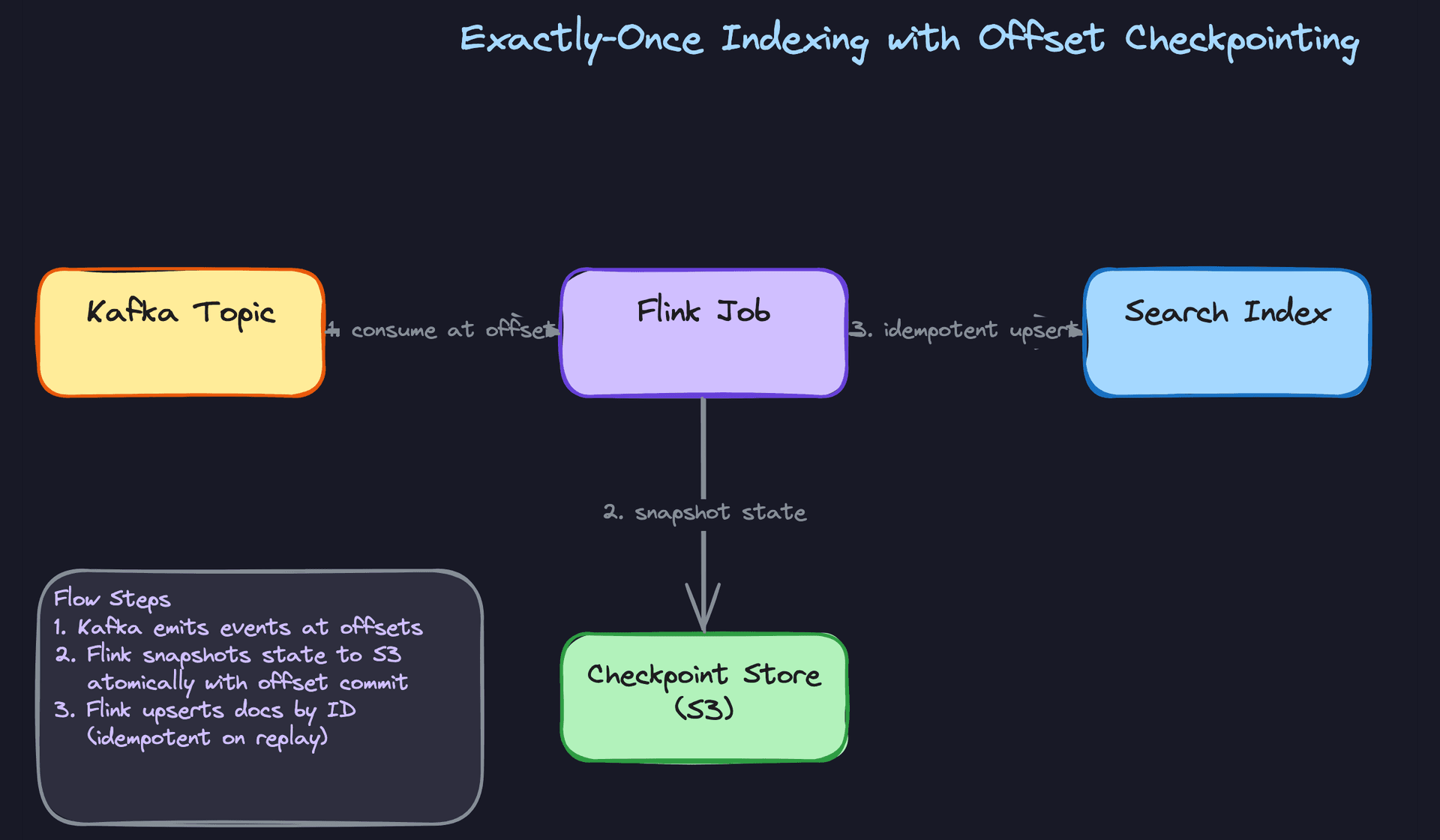
Great Solution: Flink checkpointing with atomic offset commits
Idempotent upserts handle the write side. Flink's checkpointing handles the read side. When you enable Flink checkpoints, the framework periodically snapshots all operator state, including Kafka consumer offsets, to a durable store like S3. On restart after a failure, Flink rewinds to the last successful checkpoint and replays from there.
The critical detail: Flink only advances the Kafka offset in the checkpoint after the downstream sink confirms the write. This means the offset commit and the index write are effectively atomic from a recovery standpoint.
# Flink job config (PyFlink)
env = StreamExecutionEnvironment.get_execution_environment()

# Checkpoint every 30 seconds, tolerate 1 failure before alerting
env.enable_checkpointing(30_000)
env.get_checkpoint_config().set_tolerable_checkpoint_failure_number(1)
env.get_checkpoint_config().set_checkpoint_storage("s3://my-bucket/flink-checkpoints/")

kafka_source = KafkaSource.builder() \
    .set_bootstrap_servers("kafka:9092") \
    .set_topics("document-changes") \
    .set_group_id("search-indexer") \
    .set_starting_offsets(KafkaOffsetsInitializer.committed_offsets()) \
    .set_value_only_deserializer(JsonDeserializationSchema()) \
    .build()
During a rebalance (when Kafka partitions shift between consumers), Flink pauses processing, completes the in-flight checkpoint, then resumes with the new partition assignment. You don't lose events and you don't double-write, because the idempotent upserts absorb any replays from the checkpoint boundary.
Tip: Mentioning the interaction between Flink checkpoints and Kafka rebalances is what separates senior candidates from mid-level ones. Most people know about idempotent writes. Fewer can explain what happens to in-flight events during a consumer group rebalance and why checkpointing before the rebalance matters.
"How do you handle a full index rebuild without taking search offline?"
You'll need this when you change your index mapping (adding a new field type, switching analyzers, enabling vectors) or when you've accumulated enough index drift that a clean rebuild is cheaper than patching. The naive answer kills your search availability for the duration of the rebuild.
Bad Solution: Drop and rebuild in place
Delete the existing index, create a new one with the updated mapping, run the Spark job to populate it. Simple. Also means your search API returns zero results for however long the rebuild takes. At scale, that's hours.
Some candidates try to work around this by taking the search API offline during the rebuild window. That's not a solution, that's just moving the problem.
Warning: Never propose dropping a production index as a migration strategy. The interviewer will ask "what if the rebuild job fails halfway through?" and you'll have no answer.
Good Solution: Build a shadow index, then swap
Create a new index with the updated mapping under a different name (e.g., products_v2). Run the full Spark rebuild job against it. Meanwhile, products_v1 keeps serving queries. Once the rebuild completes, validate the new index, then update the alias products to point at products_v2. The search API never touches index names directly, only the alias.
# After rebuild completes, atomically swap the alias
es_client.indices.update_aliases(
    actions=[
        {"remove": {"index": "products_v1", "alias": "products"}},
        {"add":    {"index": "products_v2", "alias": "products"}},
    ]
)
The alias swap is atomic in Elasticsearch. Queries in flight against the old index complete normally. New queries hit the new index. No downtime.
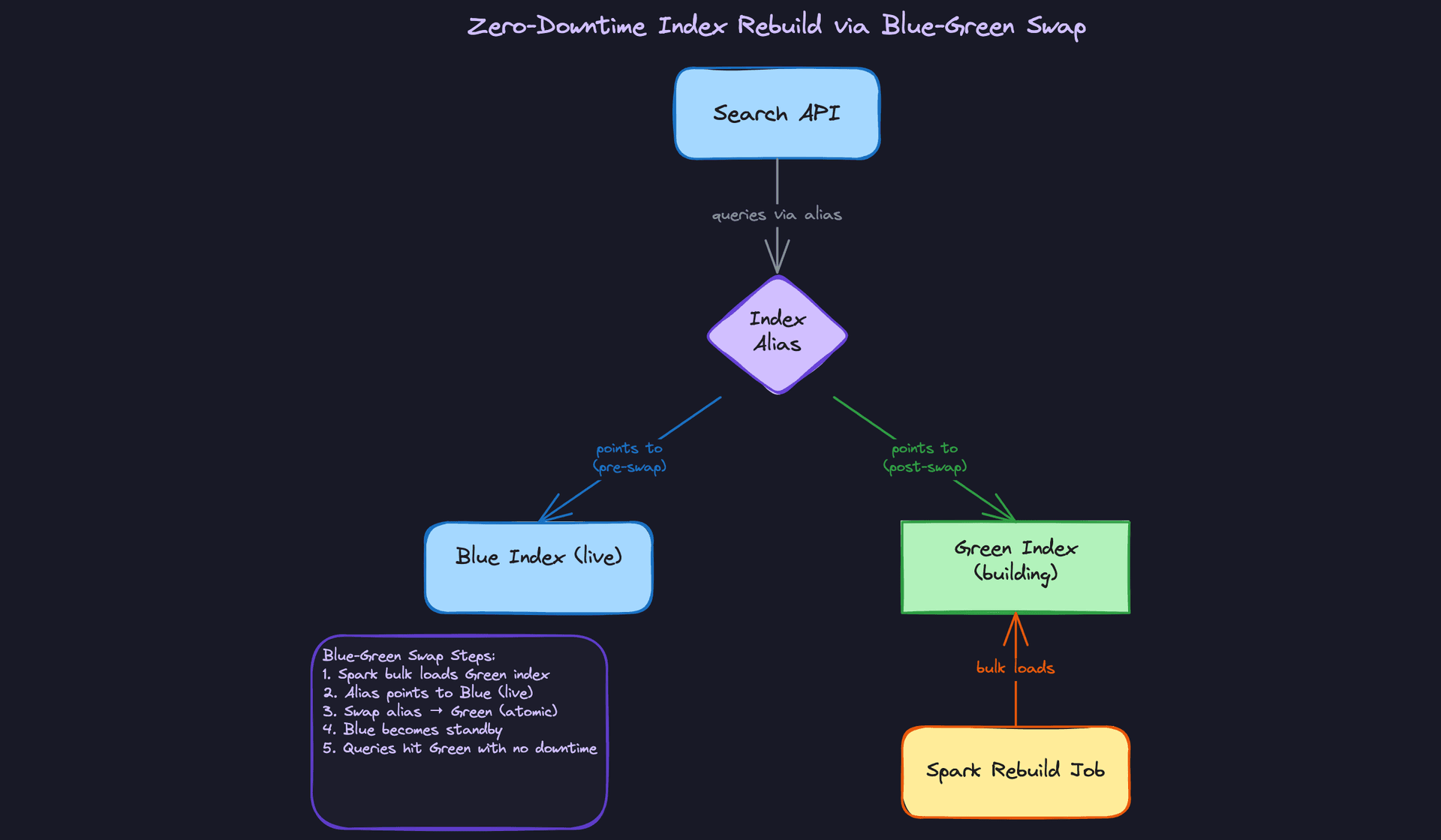
Great Solution: Blue-green swap with streaming catch-up
The shadow index approach has a gap: the rebuild takes time, and during that window new events are still arriving. When you flip the alias, products_v2 is already stale by however many hours the rebuild took.
The fix is to run the streaming indexing path against both indexes during the rebuild window. The blue index (products_v1) stays live. The green index (products_v2) gets bulk-loaded by the Spark rebuild job AND receives live streaming updates from Flink. Once the bulk load completes and the green index has caught up to the streaming offset, you flip the alias.
You validate before you swap. Check document counts, spot-check known queries, compare relevance scores on a sample query set. Only flip when you're confident.
def validate_green_index(es_client, blue: str, green: str, sample_queries: list) -> bool:
    blue_count  = es_client.count(index=blue)["count"]
    green_count = es_client.count(index=green)["count"]

    # Allow up to 0.1% variance (streaming lag)
    if abs(blue_count - green_count) / blue_count > 0.001:
        return False

    for query in sample_queries:
        blue_hits  = es_client.search(index=blue,  query=query)["hits"]["total"]["value"]
        green_hits = es_client.search(index=green, query=query)["hits"]["total"]["value"]
        if blue_hits == 0 and green_hits == 0:
            continue
        if abs(blue_hits - green_hits) / max(blue_hits, 1) > 0.05:
            return False

    return True
Keep the old index around for 24 hours after the swap. If something goes wrong, flipping the alias back is a one-line operation.
Tip: The detail about running streaming writes to both indexes during the rebuild window is what makes this answer complete. Most candidates describe the alias swap correctly but forget about the freshness gap. Bring it up before the interviewer has to ask.
"How do you scale embedding generation when it's the bottleneck in your pipeline?"
Embedding generation is expensive. A single call to a transformer model can take 50-200ms. If you're indexing millions of documents and calling an embedding service inline, your pipeline throughput collapses. This is a common problem at companies running semantic search or recommendation systems on top of their search index.
Bad Solution: Synchronous inline inference
Call the embedding service for each document inside the Flink job, wait for the response, then write to the index. Simple to implement, terrible at scale. Your pipeline throughput is now bounded by the latency and concurrency limits of the embedding service. One slow model response stalls the entire stream.
It also creates tight coupling. If the embedding service goes down, your entire indexing pipeline stops. A search infrastructure outage caused by an ML model deployment is not a good day.
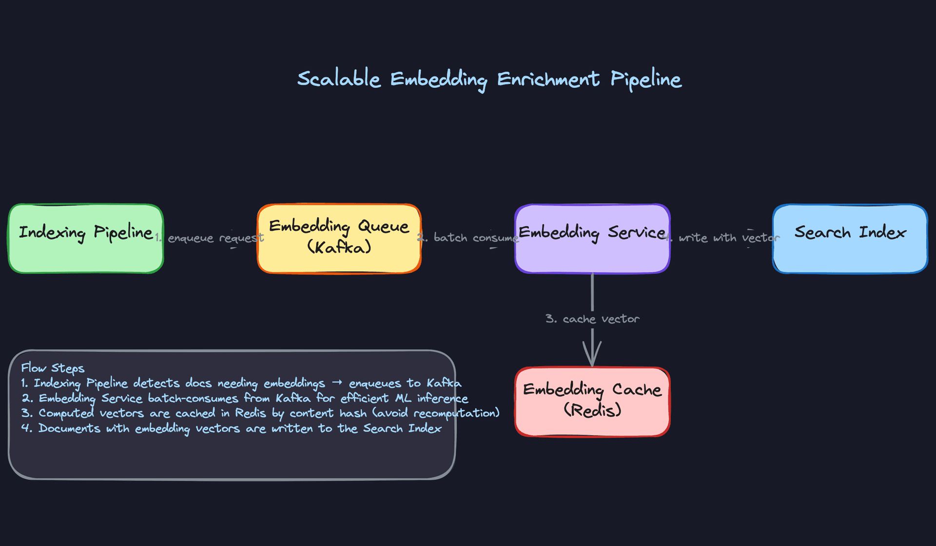
Good Solution: Batched inference with a dedicated consumer
Decouple embedding generation from the main indexing pipeline. The Flink job writes documents to a separate Kafka topic (the embedding queue) instead of calling the model directly. A dedicated embedding service consumes from that topic in batches, calls the model once per batch, and writes the enriched documents (with vector fields) back to another topic or directly to the index.
Batching matters a lot here. Most embedding models run significantly faster per document when you send 32 or 64 documents at once versus one at a time, because the GPU can parallelize across the batch.
# Embedding service consumer (simplified)
consumer = KafkaConsumer(
    "documents-pending-embedding",
    group_id="embedding-service",
    max_poll_records=64,           # batch size matches model's optimal input
)

for batch in consumer:
    texts   = [msg.value["content"] for msg in batch]
    doc_ids = [msg.value["document_id"] for msg in batch]

    vectors = embedding_model.encode(texts, batch_size=64, normalize_embeddings=True)

    for doc_id, vector in zip(doc_ids, vectors):
        es_client.update(
            index="products",
            id=doc_id,
            doc={"embedding": vector.tolist()},
        )
Great Solution: Content-hash caching plus async enrichment queue
Batching helps throughput. Caching eliminates redundant work. Many documents in a product catalog or content platform are near-duplicates: the same description with a minor edit, the same article re-published with a different slug. If you cache embeddings by a hash of the document content, you skip the model call entirely for content you've seen before.
import hashlib

def get_or_compute_embedding(content: str, cache: Redis, model) -> list[float]:
    content_hash = hashlib.sha256(content.encode()).hexdigest()
    cached = cache.get(f"emb:{content_hash}")

    if cached:
        return json.loads(cached)

    vector = model.encode([content])[0].tolist()
    cache.setex(f"emb:{content_hash}", 86400 * 7, json.dumps(vector))  # 7-day TTL
    return vector
The async enrichment queue also gives you a natural place to handle partial indexing. You can index the non-vector fields immediately (title, body, metadata) so the document is searchable right away, then update the vector field asynchronously once the embedding service processes it. Users get fast keyword search results while semantic search catches up in the background.
Tip: Proposing the two-phase index write (index now, enrich later) shows you're thinking about user-facing latency, not just pipeline throughput. That's a staff-level framing. It also naturally leads to a conversation about how you'd handle documents that never got their embeddings, which is a good data quality discussion.
"How do you monitor index freshness and catch lag before users notice?"
A pipeline that's silently behind is worse than one that's visibly broken. At least a broken pipeline pages someone. A lagging pipeline just quietly serves stale results until a user files a bug report or a business metric drops.
Bad Solution: Periodic spot checks
Run a cron job every hour that picks a random document, checks whether it's in the index, and alerts if it's missing. This catches catastrophic failures but misses the slow drift that actually hurts users: a pipeline that's 45 minutes behind on a catalog that updates every 10 minutes.
It also gives you no signal about which part of the pipeline is slow. Is the Kafka consumer falling behind? Is the enrichment step the bottleneck? Is Elasticsearch write throughput degrading? A spot check can't tell you.
Good Solution: Kafka consumer group lag metrics
Kafka exposes per-partition consumer lag natively: the difference between the latest produced offset and the last committed consumer offset. This is your primary freshness signal for the streaming path.
# Expose lag as a Prometheus metric (via kafka-consumer-groups or custom consumer)
from prometheus_client import Gauge

kafka_lag_gauge = Gauge(
    "search_indexer_kafka_lag",
    "Kafka consumer lag for search indexing pipeline",
    labelnames=["topic", "partition"],
)

def update_lag_metrics(admin_client, consumer_group: str):
    offsets = admin_client.list_consumer_group_offsets(consumer_group)
    for tp, offset_meta in offsets.items():
        end_offset = admin_client.list_offsets({tp: OffsetSpec.latest()})[tp].offset
        lag = end_offset - offset_meta.offset
        kafka_lag_gauge.labels(topic=tp.topic, partition=tp.partition).set(lag)
Alert when lag exceeds a threshold tied to your SLA. If your freshness SLA is 5 minutes and your average throughput is 10,000 events/minute, a lag of 50,000 events should page someone.
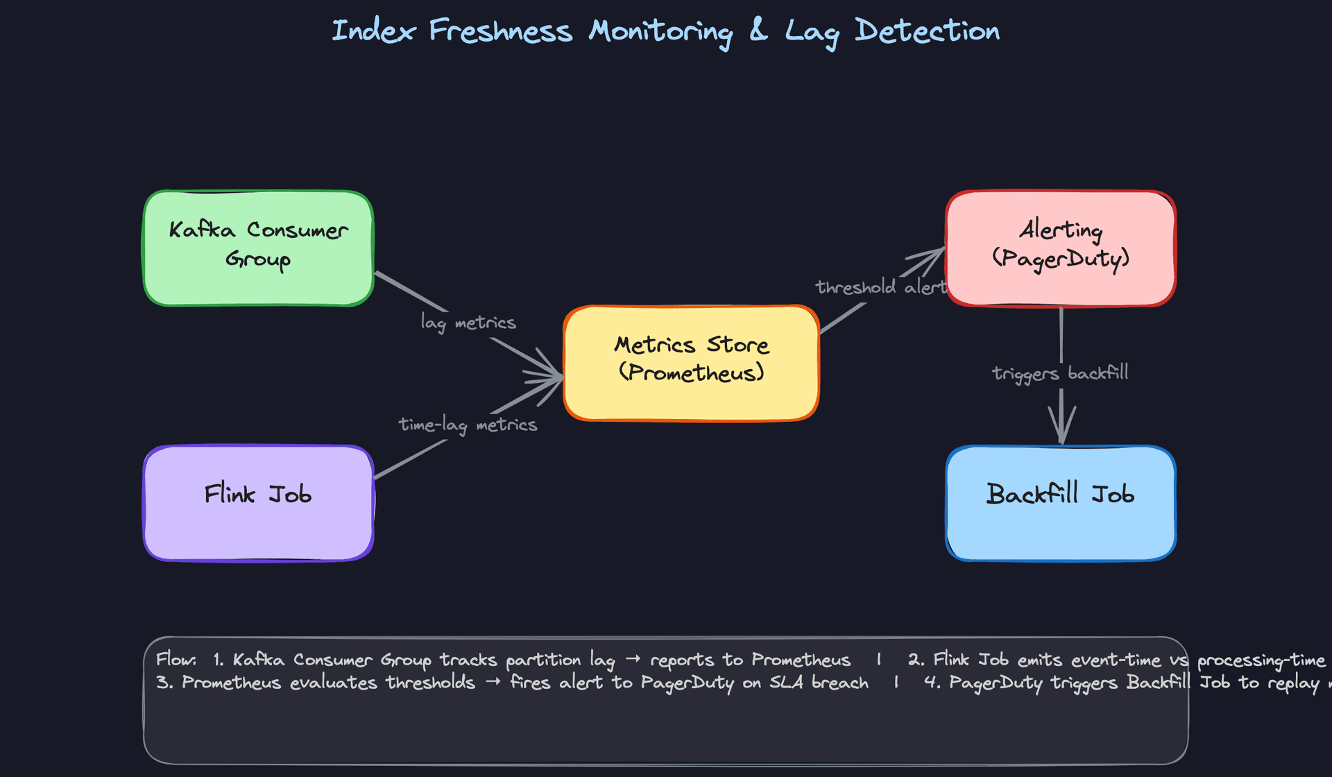
Great Solution: Event-time lag plus automated backfill
Consumer group lag tells you how many messages are waiting. Event-time lag tells you how old those messages are. These are different. A lag of 10,000 messages could be 30 seconds of backlog or 3 hours, depending on write volume.
Emit both metrics from your Flink job. Track event_time from the Kafka message versus processing_time when Flink processes it. The difference is your true freshness gap.
# Inside Flink ProcessFunction
class FreshnessMetricsFunction(ProcessFunction):
    def process_element(self, event, ctx):
        event_time_ms    = event["event_time_ms"]
        processing_time  = ctx.timer_service().current_processing_time()
        lag_seconds      = (processing_time - event_time_ms) / 1000.0

        # Emit to metrics sink (Prometheus, Datadog, etc.)
        self.metrics_group.gauge("event_processing_lag_seconds").set_value(lag_seconds)
        yield event
When lag exceeds your SLA threshold, the alerting system triggers a backfill job. For moderate lag, the backfill replays recent Kafka offsets. For severe lag (pipeline was down for hours), it reads directly from the source data lake and bulk-loads the missed window. The backfill job uses the same idempotent upsert logic as the main pipeline, so it's safe to run concurrently.
Tip: The distinction between offset lag and event-time lag is a detail most candidates skip. Bringing it up unprompted signals that you've actually operated a streaming pipeline under production conditions, not just read about one.
What is Expected at Each Level
Mid-Level
- Design the batch indexing path end-to-end: source data in object storage, Spark transformation, bulk load into Elasticsearch. You should be able to draw this without prompting.
- Explain why Kafka sits between the source system and the streaming indexer. You don't need to know Flink internals cold, but you should understand that the queue decouples ingestion speed from indexing speed.
- Identify that upserts need to be idempotent and that document ID is the natural key. If you say "just write to the index" without mentioning what happens on a pipeline restart, that's a gap.
- Handle one deep dive with some prompting. Exactly-once semantics or schema evolution are the most common. You won't be expected to drive it unprompted, but you should be able to reason through it once the interviewer opens the door.
Senior
- Proactively introduce both paths and frame the trade-off yourself. The interviewer should not have to ask "what about real-time?" You should bring it up, explain the freshness vs. operational complexity trade-off, and recommend one based on the requirements you clarified upfront.
- Drive at least two deep dives independently. Blue-green index swaps and embedding enrichment decoupling are the two most likely. If you wait to be asked, you're leaving points on the table.
- Articulate why the enrichment step must be a shared library, not duplicated logic in the batch and streaming jobs. Candidates who miss this tend to describe two separate transformation pipelines that will inevitably drift.
- Discuss shard configuration and index alias management as things you'd own alongside the search platform team, not as someone else's problem.
Staff+
- Frame the problem in terms of team ownership from the start. Who runs the search cluster? Who owns the pipeline SLA? Who gets paged when the index falls behind? These aren't organizational tangents; they determine where your design boundaries sit and what contracts you need to make explicit.
- Address multi-tenant indexing: what happens when ten product teams want to index different document types into the same cluster? You should discuss index isolation strategies, shared vs. per-tenant enrichment pipelines, and how schema versioning interacts with downstream query contracts that other teams depend on.
- Propose a concrete cost model for embedding inference. Real-time inference on every document change is expensive. Staff candidates explain when async batch inference is acceptable, how to cache embeddings by content hash, and what the latency penalty looks like for users searching freshly-created documents that haven't been embedded yet.
- Discuss how the pipeline evolves over time: what a v1 batch-only system looks like, when you add streaming, and what triggers a full architectural revisit. Interviewers at this level want to see that you think in terms of systems that grow, not systems that are designed once.
Key takeaway: The thing that separates strong candidates at every level is treating the indexing pipeline as a data contract problem, not just a throughput problem. Documents change shape, teams change requirements, and ML models change embedding dimensions. The design that survives is the one built around explicit schemas, shared transformation logic, and clear ownership boundaries from day one.
